[R] R 정리 15 - Decision Tree

# 분류모델 중 Decision Tree

set.seed(123)
ind <- sample(1:nrow(iris), nrow(iris) * 0.7, replace = FALSE)
train <- iris[ind, ]
test <- iris[-ind, ]

 

# ctree

install.packages("party")
library(party)
iris_ctree <- ctree(formula = Species ~ ., data = train)
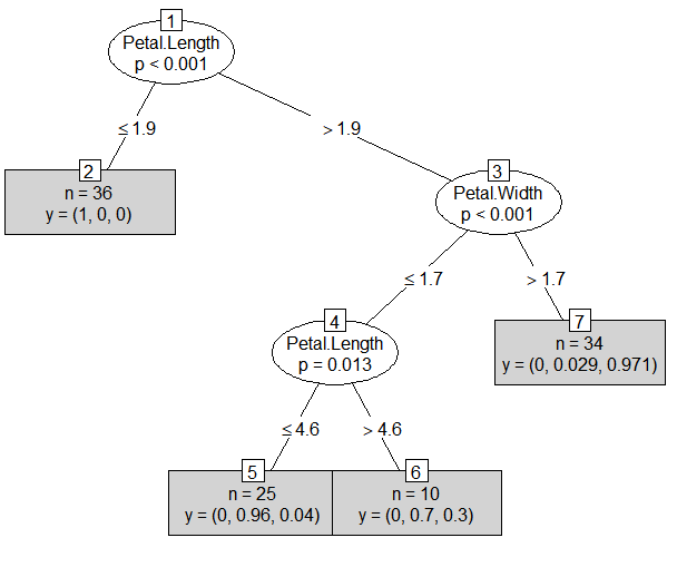
iris_ctree
# Conditional inference tree with 4 terminal nodes
# 
# Response:  Species 
# Inputs:  Sepal.Length, Sepal.Width, Petal.Length, Petal.Width 
# Number of observations:  105 
# 
# 1) Petal.Length <= 1.9; criterion = 1, statistic = 97.466
# 2)*  weights = 36 
# 1) Petal.Length > 1.9
# 3) Petal.Width <= 1.7; criterion = 1, statistic = 45.022
# 4) Petal.Length <= 4.6; criterion = 0.987, statistic = 8.721
# 5)*  weights = 25 
# 4) Petal.Length > 4.6
# 6)*  weights = 10 
# 3) Petal.Width > 1.7
# 7)*  weights = 34
plot(iris_ctree, type = "simple")
plot(iris_ctree)

 

# predit

pred <- predict(iris_ctree, test)
pred
t <- table(pred, test$Species) # 인자 : 예측값, 실제값
t
# pred         setosa versicolor virginica
# setosa         14          0         0
# versicolor      0         18         1
# virginica       0          0        12
sum(diag(t)) / nrow(test) # 0.9777778

library(caret)
confusionMatrix(pred, test$Species)
# Confusion Matrix and Statistics
# 
# Reference
# Prediction   setosa versicolor virginica
# setosa         14          0         0
# versicolor      0         18         1
# virginica       0          0        12
# 
# Overall Statistics
# 
# Accuracy : 0.9778          
# 95% CI : (0.8823, 0.9994)
# No Information Rate : 0.4             
# P-Value [Acc > NIR] : < 2.2e-16       
# 
# Kappa : 0.9662          
# 
# Mcnemar's Test P-Value : NA              
# 
# Statistics by Class:
# 
#                      Class: setosa Class: versicolor Class: virginica
# Sensitivity                 1.0000            1.0000           0.9231
# Specificity                 1.0000            0.9630           1.0000
# Pos Pred Value              1.0000            0.9474           1.0000
# Neg Pred Value              1.0000            1.0000           0.9697
# Prevalence                  0.3111            0.4000           0.2889
# Detection Rate              0.3111            0.4000           0.2667
# Detection Prevalence        0.3111            0.4222           0.2667
# Balanced Accuracy           1.0000            0.9815           0.9615

 

# 방법2 : rpart : 가지치기 이용

library(rpart)

iris_rpart <- rpart(Species ~ ., data = train, method = 'class')
x11()
plot(iris_rpart)
text(iris_rpart)

plotcp(iris_rpart)
printcp(iris_rpart)

cp <- iris_rpart$cptable[which.min(iris_rpart$cptable[, 'xerror'])]
iris_rpart_prune <- prune(iris_rpart, cp=cp, 'cp')
x11()
plot(iris_rpart_prune)
text(iris_rpart_prune)