BACK END/R
[R] R 정리 23 - 비계층적 군집분석2 (k-means)
circle kim
2021. 2. 5. 11:23
23. 계층적 분집분석 : k-means
- data load
data <- read.csv("testdata/exam.csv", sep = " ")
data
#     bun kor mat eng sci
# 1    1  98  95  95  90
# 2    2  65  90  60  88
# 3    3  85  53  48  50
# 4    4  65  92  62  90
# 5    5  68  72  88  73
# 6    6  90  92  90  96
# 7    7  65  70  76  80
# 8    8  60  91  62  90
# 9    9  65  70  86  76
# 10  10 100  98  97 100
- 거리계산
d_data <- dist(data, method = "euclidean")
d_data
#            1         2         3         4         5         6         7         8         9
# 2  48.414874
# 3  75.802375 57.948253
# 4  46.861498  4.000000 60.975405
# 5  42.225585 36.755952 52.754147 37.080992
# 6  12.609520 40.112342 73.722452 38.065733 37.656341
# 7  47.021272 27.294688 48.877398 28.089144 14.491377 39.522146
# 8  50.970580  8.366600 62.369865  6.480741 37.403208 41.533119 27.622455
# 9  45.332108 35.623026 53.338541 35.791060  6.480741 39.166312 10.954451 35.199432
# 10 14.071247 53.535035 84.852814 51.205468 50.348784 14.730920 53.469618 54.571055 52.028838
- 다차원 척도법
gra_data <- cmdscale(d_data)
gra_data
plot(gra_data, type = "n") # 그래프 분석 시 4개의 군집 확인 가능
text(gra_data, as.character(1:10)) # 그래프에 text 출력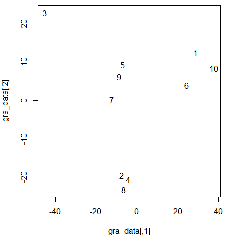
data$avg <- apply(data[, 2:5], 1, mean) # 참고용 avg - data에 행으로 mean() 함수 수행
data
#    bun kor mat eng sci   avg
# 1    1  98  95  95  90 94.50
# 2    2  65  90  60  88 75.75
# 3    3  85  53  48  50 59.00
# 4    4  65  92  62  90 77.25
# 5    5  68  72  88  73 75.25
# 6    6  90  92  90  96 92.00
# 7    7  65  70  76  80 72.75
# 8    8  60  91  62  90 75.75
# 9    9  65  70  86  76 74.25
# 10  10 100  98  97 100 98.75
- k-means
library(NbClust)
data_s <- scale(data[2:5])
head(data_s)
#             kor        mat        eng        sci
# [1,]  1.4199308  0.8523469  1.0794026  0.4640535
# [2,] -0.7196910  0.5167772 -0.9517313  0.3255301
# [3,]  0.5770495 -1.9664380 -1.6481201 -2.3064152
# [4,] -0.7196910  0.6510051 -0.8356665  0.4640535
# [5,] -0.5251799 -0.6912734  0.6731758 -0.7133957
# [6,]  0.9012346  0.6510051  0.7892406  0.8796238
- Best 군집 수 획득
nc <- NbClust::NbClust(data_s, min.nc = 2, max.nc = 5, method = "kmeans")
nc # 4 2 3 2 1 4 1 2 1 4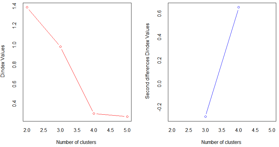
plot(table(nc$Best.nc[1,]))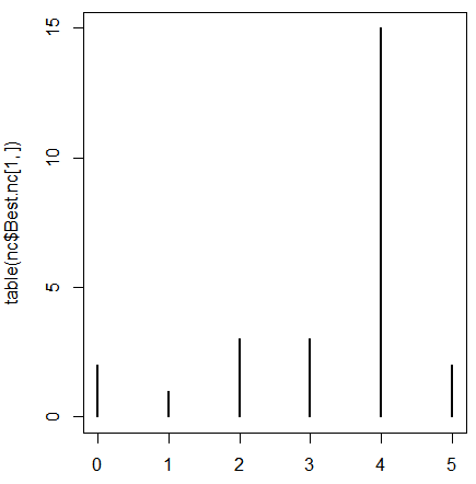
- model
model_kmeans <- kmeans(data[, c("bun", "avg")], 4)
model_kmeans

table(model_kmeans$cluster)
# 1 2 3 4
# 3 1 3 3

cluster <- model_kmeans$cluster
cluster # 2 1 4 1 1 2 3 3 3 2
kmeans_df <- cbind(cluster, data[, c("bun", "avg")])
kmeans_df
#    cluster bun   avg
# 1        4   1 94.50
# 2        1   2 75.75
# 3        3   3 59.00
# 4        1   4 77.25
# 5        1   5 75.25
# 6        4   6 92.00
# 7        2   7 72.75
# 8        2   8 75.75
# 9        2   9 74.25
# 10       4  10 98.75

str(kmeans_df)
kmeans_df <- transform(kmeans_df, cluster = as.factor(cluster)) # 범주형으로 변경
str(kmeans_df)
- clustering
library(ggplot2)
df_plot <- ggplot(data = kmeans_df, aes(x=bun, y=avg, col = cluster)) +
            geom_point(aes(shape=factor(cluster), size = 4)) +
            ggtitle("군집분석연습")
df_plot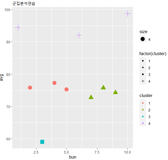
- 계층적 군집분석 : k -means
data("diamonds")
diamonds
# carat cut       color clarity depth table price     x     y     z
# <dbl> <ord>     <ord> <ord>   <dbl> <dbl> <int> <dbl> <dbl> <dbl>
#   1 0.23  Ideal     E     SI2      61.5    55   326  3.95  3.98  2.43
# 2 0.21  Premium   E     SI1      59.8    61   326  3.89  3.84  2.31
# 3 0.23  Good      E     VS1      56.9    65   327  4.05  4.07  2.31
# 4 0.290 Premium   I     VS2      62.4    58   334  4.2   4.23  2.63
# 5 0.31  Good      J     SI2      63.3    58   335  4.34  4.35  2.75
# 6 0.24  Very Good J     VVS2     62.8    57   336  3.94  3.96  2.48
# 7 0.24  Very Good I     VVS1     62.3    57   336  3.95  3.98  2.47
# 8 0.26  Very Good H     SI1      61.9    55   337  4.07  4.11  2.53
# 9 0.22  Fair      E     VS2      65.1    61   337  3.87  3.78  2.49
# 10 0.23  Very Good H     VS1      59.4    61   338  4     4.05  2.39
typeof(diamonds) # list

length(diamonds) # 10
NROW(diamonds) # 53940
t <- sample(1:nrow(diamonds), 1000)
test <- diamonds[t, ]
dim(test) # 1000   10
str(test)

mydia <- test[c("price", "carat","depth","table")]
head(mydia)
1. 계층적 군집분석(탐색적)
result1 <- hclust(dist(mydia), method = "ave")
result1
plot(result1, hang = -1)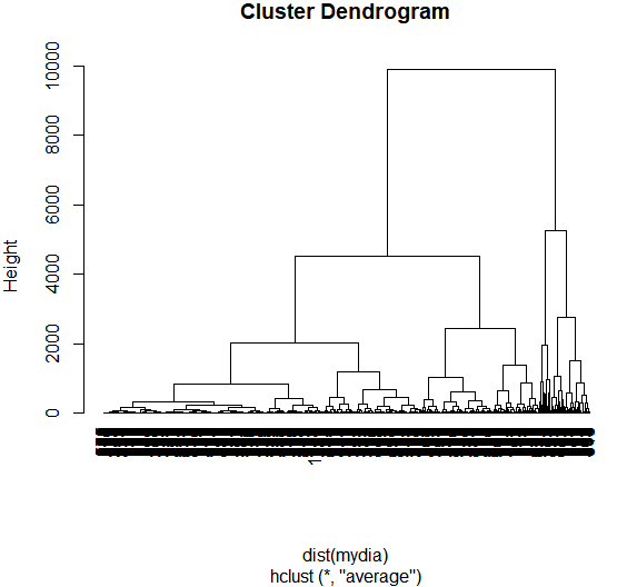
2. 비계층적 군집분석(확인적)
result2 <- kmeans(mydia, 4) # 군집 수 4
result2
names(result2)

result2$cluster

mydia$cluster <- result2$cluster
head(mydia)
#     price carat depth table cluster
# <int> <dbl> <dbl> <dbl>   <int>
#   1 11322  1.7   60.1    58       1
# 2  1009  0.5   63.8    57       3
# 3  1022  0.43  62.4    60       3
# 4  4778  1.2   58.5    61       4
# 5  4111  0.81  61.6    58       4
# 6   675  0.3   61.3    60       3

cor(mydia[, -5], method = 'pearson') # 상관계수
#             price      carat       depth      table
# price  1.00000000 0.90263800 -0.01329869  0.1134894
# carat  0.90263800 1.00000000  0.02856267  0.1670910
# depth -0.01329869 0.02856267  1.00000000 -0.3562396
# table  0.11348941 0.16709103 -0.35623960  1.0000000

plot(mydia[, -5])

plot(mydia[c("carat", "price")], col=mydia$cluster) # price과 carat열로 군집 결과 시각화

# 중심점 표시
points(result2$centers[, c("carat", "price")], col = c(1,2,3,4), pch=8, cex=5)