단순선형 회귀 Simple Linear Regression
: ols()
: 독립변수 - 연속형, 종속변수 - 연속형.
: 독립변수 1개
* linear_reg4.py
import pandas as pd
import numpy as np
import matplotlib.pyplot as plt
plt.rc('font', family='malgun gothic')

df = pd.read_csv('../testdata/drinking_water.csv')
print(df.head(3), '\n', df.describe())
'''
   친밀도  적절성  만족도
0    3    4    3
1    3    3    2
2    4    4    4
'''

print(df.corr()) # 적절성/만족도 상관계수 : 0.766853

print('----------------------------------------------------------------------')
import statsmodels.formula.api as smf

model = smf.ols(formula='만족도 ~ 적절성', data=df).fit()
print(model.summary())
OLS Regression Results
==============================================================================
Dep. Variable: 만족도 R-squared: 0.588
Model: OLS Adj. R-squared: 0.586
Method: Least Squares F-statistic: 374.0
Date: Thu, 11 Mar 2021 Prob (F-statistic): 2.24e-52
Time: 10:07:49 Log-Likelihood: -207.44
No. Observations: 264 AIC: 418.9
Df Residuals: 262 BIC: 426.0
Df Model: 1
Covariance Type: nonrobust
==============================================================================
coef std err t P>|t| [0.025 0.975]
------------------------------------------------------------------------------
Intercept 0.7789 0.124 6.273 0.000 0.534 1.023
적절성 0.7393 0.038 19.340 0.000 0.664 0.815
==============================================================================
Omnibus: 11.674 Durbin-Watson: 2.185
Prob(Omnibus): 0.003 Jarque-Bera (JB): 16.003
Skew: -0.328 Prob(JB): 0.000335
Kurtosis: 4.012 Cond. No. 13.4
==============================================================================
Notes:
[1] Standard Errors assume that the covariance matrix of the errors is correctly specified.[해석]
상관계수 ** 2 = 결정계수
print(0.766853 ** 2) # 0.588063523609
R-squared : 결정계수(설명력), 상관계수 R의 제곱 : 0.588
: 1 - (SSE(explain sum of square-추세선과 데이터간 y값) / SST(total sum of square - 평균과 추세선간 y값
차이) )
: 1 - (SSE / SST)
=> over fitting : R2가 1에 아주 가까우면(기존 데이터와 추사) 새로운 데이터에 대해 설명력이 좋지않다.
적절성의 p-value : 0.000 < 0.05 => 모델은 유효하다.
std err(표준 오차) : 0.038
Intercept(y절편) : 0.7789
coef(기울기) : 0.7393
t = 기울기/ 표준오차 : 19.340
print(0.7393 / 0.038) # 19.455263157894738
F-statistic = t**2 : 374.0
print(19.340 ** 2) # 374.0356
독립변수가 많을 경우 R-squared과 Adj. R-squared의 차이가 클 경우 독립변수 이상치를 확인해야한다.
Kurtosis : 4.012 => 3보다 클경우 평균에 데이터가 몰려있다.

print(model.params) # y절편과 기울기 산출
# Intercept    0.778858
#적절성          0.739276

print(model.rsquared) # 0.5880630629464404
print()
print(model.pvalues)
'''
Intercept    1.454388e-09
적절성          2.235345e-52
'''
#print(model.predict()) # 예측값
print(df.만족도[0],' ', model.predict()[0]) # 3   3.7359630488589186

# 새로운 값 예측
print(df.적절성[:5])
'''
3   3.7359630488589186
0    4
1    3
2    4
3    2
4    2
'''

print(df.만족도[:5])
'''
0    3
1    2
2    4
3    2
4    2
'''

print(model.predict()[:5]) # [3.73596305 2.99668687 3.73596305 2.25741069 2.25741069]
print()

new_df = pd.DataFrame({'적절성':[6,5,4,3,22]})
new_pred = model.predict(new_df)
print('new_pred :\n', new_pred)
'''
 0     5.214515
1     4.475239
2     3.735963
3     2.996687
4    17.042934
'''

plt.scatter(df.적절성, df.만족도)
slope, intercept = np.polyfit(df.적절성, df.만족도, 1) # R의 abline 기능
plt.plot(df.적절성, df.적절성 * slope + intercept, 'b') # 추세선
plt.show()
다중 선형회귀 Multiple Linear Regression
: 독립변수가 복수
model2 = smf.ols(formula='만족도 ~ 적절성 + 친밀도', data=df).fit()
print(model2.summary())
OLS Regression Results
==============================================================================
Dep. Variable: 만족도 R-squared: 0.598
Model: OLS Adj. R-squared: 0.594
Method: Least Squares F-statistic: 193.8
Date: Thu, 11 Mar 2021 Prob (F-statistic): 2.61e-52
Time: 11:19:33 Log-Likelihood: -204.37
No. Observations: 264 AIC: 414.7
Df Residuals: 261 BIC: 425.5
Df Model: 2
Covariance Type: nonrobust
==============================================================================
coef std err t P>|t| [0.025 0.975]
------------------------------------------------------------------------------
Intercept 0.6673 0.131 5.096 0.000 0.409 0.925
적절성 0.6852 0.044 15.684 0.000 0.599 0.771
친밀도 0.0959 0.039 2.478 0.014 0.020 0.172
==============================================================================
Omnibus: 13.103 Durbin-Watson: 2.174
Prob(Omnibus): 0.001 Jarque-Bera (JB): 17.256
Skew: -0.382 Prob(JB): 0.000179
Kurtosis: 3.992 Cond. No. 18.8
==============================================================================
Notes:
[1] Standard Errors assume that the covariance matrix of the errors is correctly specified.단순 선형 회귀
: iris dataset, ols() 사용. 상관관계가 약한/강한 변수로 모델 작성.
* linear_reg5.py
import pandas as pd
import statsmodels.formula.api as smf
import seaborn as sns
iris = sns.load_dataset('iris')
print(iris.head(3))
'''
   sepal_length  sepal_width  petal_length  petal_width species
0           5.1          3.5           1.4          0.2  setosa
1           4.9          3.0           1.4          0.2  setosa
2           4.7          3.2           1.3          0.2  setosa
'''

print(iris.corr())
'''
              sepal_length  sepal_width  petal_length  petal_width
sepal_length      1.000000    -0.117570      0.871754     0.817941
sepal_width      -0.117570     1.000000     -0.428440    -0.366126
petal_length      0.871754    -0.428440      1.000000     0.962865
petal_width       0.817941    -0.366126      0.962865     1.000000
'''
# 단순 선형회귀 모델 : 상관관계 r = -0.117570(sepal_length/sepal_width)
result = smf.ols(formula = 'sepal_length ~ sepal_width', data=iris).fit()
#print(result.summary()) # R2 : 0.014
print(result.rsquared)# 0.01382 < 0.05 => 의미없는 모델
print(result.pvalues) # 1.518983e-01 > 0.05result2 = smf.ols(formula = 'sepal_length ~ petal_length', data=iris).fit()
print(result2.summary()) # R2 : 0.760 => 설명력
print(result2.rsquared)# 0.7599 > 0.05 => 의미있는 모델
print(result2.pvalues) # 1.038667e-47 < 0.05
print()
pred = result2.predict()
print('실제값 :', iris.sepal_length[0]) # 실제값 : 5.1
print('예측값 :', pred[0]) # 예측값 : 4.879094603339241
# 새로운 데이터로 예측
print(iris.petal_length[1:5])
new_data = pd.DataFrame({'petal_length':[1.4, 0.5, 8.5, 12.123]})
print(new_data)
'''
petal_length
0 1.400
1 0.500
2 8.500
3 12.123
'''
y_pred_new = result2.predict(new_data)
print('새로운 데이터로 sepal_length예측 :\n', y_pred_new)
'''
0 4.879095
1 4.511065
2 7.782443
3 9.263968
'''
다중 선형 회귀
result3 = smf.ols(formula = 'sepal_length ~ petal_length + petal_width', data=iris).fit()
print(result3.summary()) #  R2 : 0.760      => 설명력
OLS Regression Results
==============================================================================
Dep. Variable: sepal_length R-squared: 0.766
Model: OLS Adj. R-squared: 0.763
Method: Least Squares F-statistic: 241.0
Date: Thu, 11 Mar 2021 Prob (F-statistic): 4.00e-47
Time: 12:09:43 Log-Likelihood: -75.023
No. Observations: 150 AIC: 156.0
Df Residuals: 147 BIC: 165.1
Df Model: 2
Covariance Type: nonrobust
================================================================================
coef std err t P>|t| [0.025 0.975]
--------------------------------------------------------------------------------
Intercept 4.1906 0.097 43.181 0.000 3.999 4.382
petal_length 0.5418 0.069 7.820 0.000 0.405 0.679
petal_width -0.3196 0.160 -1.992 0.048 -0.637 -0.002
==============================================================================
Omnibus: 0.383 Durbin-Watson: 1.826
Prob(Omnibus): 0.826 Jarque-Bera (JB): 0.540
Skew: 0.060 Prob(JB): 0.763
Kurtosis: 2.732 Cond. No. 25.3
==============================================================================print('R-squared :', result3.rsquared)# 0.7662 > 0.05 => 의미있는 모델
print('p-value', result3.pvalues)
# petal_length 9.414477e-13
# petal_width 4.827246e-02
# y = 0.5418 * x1 -0.3196 * x2 + 4.1906# 새로운 데이터로 예측
new_data2 = pd.DataFrame({'petal_length':[8.5, 12.12], 'petal_width':[8.5, 12.5]})
y_pred_new2 = result3.predict(new_data2)
print('새로운 데이터로 sepal_length예측 :\n', y_pred_new2)
'''
0 6.079508
1 6.762540
'''
선형 회귀 분석
: mtcars dataset, ols() 사용. 모델작성 후 추정치 얻기
* linear_reg6.py
import statsmodels.api
import statsmodels.formula.api as smf
import numpy as np
import pandas as pd
import matplotlib.pyplot as plt

plt.rc('font', family='malgun gothic')

mtcars = statsmodels.api.datasets.get_rdataset('mtcars').data
print(mtcars)
'''
                      mpg  cyl   disp   hp  drat  ...   qsec  vs  am  gear  carb
Mazda RX4            21.0    6  160.0  110  3.90  ...  16.46   0   1     4     4
Mazda RX4 Wag        21.0    6  160.0  110  3.90  ...  17.02   0   1     4     4
'''
print(mtcars.columns) # Index(['mpg', 'cyl', 'disp', 'hp', 'drat', 'wt', 'qsec', 'vs', 'am', 'gear', 'carb'], dtype='object')
print(mtcars.describe())
print(np.corrcoef(mtcars.hp, mtcars.mpg)) # 상관계수 : -0.77616837
print(np.corrcoef(mtcars.wt, mtcars.mpg)) # 상관계수 : -0.86765938
print(mtcars.corr())
# 시각화
plt.scatter(mtcars.hp, mtcars.mpg)
plt.xlabel('마력 수')
plt.ylabel('연비')
slope, intercept = np.polyfit(mtcars.hp, mtcars.mpg, 1) # 1차원
plt.plot(mtcars.hp, mtcars.hp * slope + intercept, 'r')
plt.show()
# 단순선형 회귀
result = smf.ols('mpg ~ hp', data=mtcars).fit()
print(result.summary())
print(result.conf_int(alpha=0.05)) # 33.435772
print(result.summary().tables[0])  # coef * x + Intercept
print('마력수  110에 대한 연비 예측 :', -0.0682 * 110 + 30.0989) # 22.5969
print('마력수  50에 대한 연비 예측 :', -0.0682 * 50 + 30.0989)   # 26.6889
# 마력이 증가하면 연비는 줄어든다. 음의 상관관계이므로 결과는 반비례한다. 참고 자료로만 활용해야한다.
# 다중선형 회귀
result2 = smf.ols('mpg ~ hp + wt', data=mtcars).fit()
print(result2.summary())
print(result2.conf_int(alpha=0.05))
print(result2.summary().tables[0])
print('마력수 110 + 무게 5에 대한 연비 예측 :', ((-0.0318 * 110) +(-3.8778 * 5) + 37.2273)) # 14.3403print('추정치 구하기 차체 무게를 입력해 연비를 추정')
result3 = smf.ols('mpg ~ wt', data=mtcars).fit()
print(result3.summary())
print('결정계수 :', result3.rsquared) # 0.7528327936582646 > 0.05 설명력이 우수한 모델
pred = result3.predict()# 1개의 자료로 실제값과 예측값(추정값) 저장 후 비교
print(mtcars.mpg[0])
print(pred[0]) # 모든 자동차 차체 무게에 대한 연비 추정치 출력
data = {
'mpg':mtcars.mpg,
'mpg_pred':pred
}
df = pd.DataFrame(data)
print(df)
'''
mpg mpg_pred
Mazda RX4 21.0 23.282611
Mazda RX4 Wag 21.0 21.919770
Datsun 710 22.8 24.885952
'''# 새로운 차체 무게로 연비 추정하기
mtcars.wt = float(input('차체 무게 입력:'))
new_pred = result3.predict(pd.DataFrame(mtcars.wt))
print('차체 무게 {}일때 예상연비{}이다'.format(mtcars.wt[0], new_pred[0]))
# 차체 무게 1일때 예상연비31.940654594619367이다# 여러 차제 무게에 대한 연비 추정
new_wt = pd.DataFrame({'wt':[6, 3, 0.5]})
new_pred2 = result3.predict(pd.DataFrame(new_wt))
print('예상연비 : \n', np.round(new_pred2.values, 2)) # [ 5.22 21.25 34.61]선형 회귀 분석
: 여러매체의 광고비에 따른 판매량 데이터, ols() 사용. 모델작성 후 추정치 얻기
* linear_reg7
import statsmodels.api
import statsmodels.formula.api as smf
import numpy as np
import pandas as pd
import matplotlib.pyplot as plt


adf_df = pd.read_csv('../testdata/Advertising.csv', usecols=[1,2,3,4])
print(adf_df.head(3), ' ', adf_df.shape) # (200, 4)
print(adf_df.index, adf_df.columns)
print(adf_df.info())
'''
      tv  radio  newspaper  sales
0  230.1   37.8       69.2   22.1
1   44.5   39.3       45.1   10.4
2   17.2   45.9       69.3    9.3
'''

print('상관계수 r : \n', adf_df.loc[:, ['sales', 'tv']].corr())
'''
           sales        tv
sales  1.000000  0.782224
tv     0.782224  1.000000
'''
# r : 0.782224 > 0.05 => 강한 양의 상관관계이고, 인과관계임을 알 수 있다.
print()

lm = smf.ols(formula='sales ~ tv', data=adf_df).fit()
print(lm.summary()) # R-squared : 0.612, p : 1.47e-42
print(lm.params)
print(lm.pvalues)
print(lm.rsquared)
# 시각화
plt.scatter(adf_df.tv, adf_df.sales)
plt.xlabel('tv')
plt.ylabel('sales')
x = pd.DataFrame({'tv':[adf_df.tv.min(), adf_df.tv.max()]})
y_pred = lm.predict(x)
plt.plot(x, y_pred, c='red')
plt.title('Linear Regression')
sns.regplot(adf_df.tv, adf_df.sales, scatter_kws = {'color':'r'})
plt.xlim(-50, 350)
plt.ylim(ymin=0)
plt.show()
# 예측 : 새로운 tv값으로 sales를 추정
x_new = pd.DataFrame({'tv':[230.1, 44.5, 100]})
pred = lm.predict(x_new)
print('추정값 :\n', pred)
'''
0    17.970775
1     9.147974
2    11.786258
'''
print('\n다중 선형회귀 모델 ')
lm_mul = smf.ols(formula = 'sales ~ tv + radio + newspaper', data = adf_df).fit()
# + newspaper 포함시와 미포함시의 R2값 변화가 없어 제거 필요.
print(lm_mul.summary())
print(adf_df.corr())
# 예측2 : 새로운 tv, radio값으로 sales를 추정
x_new2 = pd.DataFrame({'tv':[230.1, 44.5, 100], 'radio':[30.1, 40.1, 50.1],\
'newspaper':[10.1, 10.1, 10.1]})
pred2 = lm.predict(x_new2)
print('추정값 :\n', pred2)
'''
0 17.970775
1 9.147974
2 11.786258
'''회귀분석모형의 적절성을 위한 조건
: 아래의 조건 위배 시에는 변수 제거나 조정을 신중히 고려해야 함.
- 정규성 : 독립변수들의 잔차항이 정규분포를 따라야 한다.
- 독립성 : 독립변수들 간의 값이 서로 관련성이 없어야 한다.
- 선형성 : 독립변수의 변화에 따라 종속변수도 변화하나 일정한 패턴을 가지면 좋지 않다.
- 등분산성 : 독립변수들의 오차(잔차)의 분산은 일정해야 한다. 특정한 패턴 없이 고르게 분포되어야 한다.
- 다중공선성 : 독립변수들 간에 강한 상관관계로 인한 문제가 발생하지 않아야 한다.
# 잔차항
fitted = lm_mul.predict(adf_df)     # 예측값
print(fitted)
'''
0      20.523974
1      12.337855
2      12.307671
'''
residual = adf_df['sales'] - fitted # 잔차

import seaborn as sns
print('선형성 - 예측값과 잔차가 비슷하게 유지')
sns.regplot(fitted, residual, lowess = True, line_kws = {'color':'red'})
plt.plot([fitted.min(), fitted.max()], [0, 0], '--', color='grey')
plt.show() # 선형성을 만족하지 못한다. 
print('정규성- 잔차가 정규분포를 따르는 지 확인')
import scipy.stats as stats
sr = stats.zscore(residual)
(x, y), _ = stats.probplot(sr)
sns.scatterplot(x, y)
plt.plot([-3, 3], [-3, 3], '--', color="grey")
plt.show() # 선형성을 만족하지 못한다.
print('residual test :', stats.shapiro(residual))
# residual test : ShapiroResult(statistic=0.9176644086837769, pvalue=3.938041004403203e-09)
# pvalue=3.938041004403203e-09 < 0.05 => 정규성을 만족하지못함.
print('독립성 - 잔차가 자기상관(인접 관측치의 오차가 상관되어 있음)이 있는지 확인')
# 모델.summary() Durbin-Watson:2.084 => 잔차항이 독립성을 만족하는 지 확인. 2에 가까우면 자기상관이 없다.(서로 독립- 잔차끼리 상관관계가 없다)
# 0에 가까우면 양의 상관, 4에 가까우면 음의 상관.
print('등분산성 - 잔차의 분산이 일정한지 확인')
sns.regplot(fitted, np.sqrt(np.abs(sr)), lowess = True, line_kws = {'color':'red'})
plt.show()
# 추세선이 수평선을 그리지않으므로 등분산성을 만족하지 못한다.
print('다중공선성 - 독립변수들 간에 강한 상관관계 확인')
# VIF(Variance Inflation Factors - 분산 팽창 요인) 값이 10을 넘으면 다중공선성이 발생하는 변수라고 할 수 있다.
from statsmodels.stats.outliers_influence import variance_inflation_factor
print(variance_inflation_factor(adf_df.values, 0)) # 23.198876299003153
print(variance_inflation_factor(adf_df.values, 1)) # 12.570312383503682
print(variance_inflation_factor(adf_df.values, 2)) # 3.1534983754953845
print(variance_inflation_factor(adf_df.values, 3)) # 55.3039198336228

# DataFrame으로 보기
vif_df = pd.DataFrame()
vif_df['vid_value'] = [variance_inflation_factor(adf_df.values, i) for i in range(adf_df.shape[1])]
print(vif_df)
'''
   vid_value
0  23.198876
1  12.570312
2   3.153498
3  55.303920
'''
print('참고 : cooks distance - 극단값을 나타내는 지료 확인')
from statsmodels.stats.outliers_influence import OLSInfluence
cd, _ = OLSInfluence(lm_mul).cooks_distance
print(cd.sort_values(ascending=False).head())
'''
130 0.272956
5 0.128306
75 0.056313
35 0.051275
178 0.045921
'''
import statsmodels.api as sm
sm.graphics.influence_plot(lm_mul, criterion='cooks')
plt.show()
print(adf_df.iloc[[130, 5, 75, 35, 178]]) # 극단 값으로 작업에서 제외 권장.
'''
        tv  radio  newspaper  sales
130    0.7   39.6        8.7    1.6
5      8.7   48.9       75.0    7.2
75    16.9   43.7       89.4    8.7
35   290.7    4.1        8.5   12.8
178  276.7    2.3       23.7   11.8
'''
* linear_reg8.py
from sklearn.linear_model import LinearRegression
import statsmodels.api

mtcars = statsmodels.api.datasets.get_rdataset('mtcars').data
print(mtcars[:3])
'''
                mpg  cyl   disp   hp  drat     wt   qsec  vs  am  gear  carb
Mazda RX4      21.0    6  160.0  110  3.90  2.620  16.46   0   1     4     4
Mazda RX4 Wag  21.0    6  160.0  110  3.90  2.875  17.02   0   1     4     4
Datsun 710     22.8    4  108.0   93  3.85  2.320  18.61   1   1     4     1
'''

# hp(마력수)가 mpg(연비)에 영향을 미치지는 지, 인과관계가 있다면 연비에 미치는 영향값(추정치, 예측치)을 예측 (정량적 분석)
x = mtcars[['hp']].values
y = mtcars[['mpg']].values
print(x[:3])
'''
[[110]
 [110]
 [ 93]]
'''
print(y[:3])
'''
[[21. ]
 [21. ]
 [22.8]]
'''

import matplotlib.pyplot as plt
plt.scatter(x, y) # 산포도 출력
plt.show()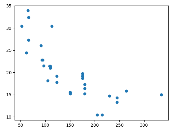
fit_model = LinearRegression().fit(x, y)   # 모델 생성
print('slope :', fit_model.coef_[0])       # 기울기 : [-0.06822828]
print('intercept :', fit_model.intercept_) # y절편 : [30.09886054]
# newY = fit_model.coef_[0] * newX + fit_model.intercept_

pred = fit_model.predict(x)
print(pred[:3])
print('예측값 :', pred[:3].flatten()) # 예측값 : [22.59374995 22.59374995 23.75363068]
print('실제값 :', y[:3].flatten())    # 실제값 : [21.  21.  22.8]
print()

# 모델 성능 파악 시 R2 또는 RMSE
from sklearn.metrics import mean_squared_error
import numpy as np

lin_mse = mean_squared_error(y, pred)   # 평균 제곱 오차
lin_rmse = np.sqrt(lin_mse)             # 루트
print("평균 제곱 오차 : ", lin_mse)          # 평균 제곱 오차 :  13.989822298268805
print("평균 제곱근 편차(RMSE) : ", lin_rmse) # 평균 제곱근 편차(RMSE) :  3.7402970868994894
print()

# 마력에 따른 연비 추정치
new_hp = [[100]]
new_pred = fit_model.predict(new_hp)
print('%s 마력인 경우 연비 추정치는 %s'%(new_hp[0][0], new_pred[0][0]))
# 100 마력인 경우 연비 추정치는 23.27603273246613
선형회귀 분석 : Linear Regression
과적합 방지를 위해 Ridgo, Lasso, ElasticNet
* linear_reg9.py
import numpy as np
import pandas as pd
from sklearn.datasets import load_iris

iris = load_iris()
print(iris)
'''
[[5.1, 3.5, 1.4, 0.2],
[4.9, 3. , 1.4, 0.2],
[4.7, 3.2, 1.3, 0.2],
[4.6, 3.1, 1.5, 0.2],
[5. , 3.6, 1.4, 0.2],
[5.4, 3.9, 1.7, 0.4],
[4.6, 3.4, 1.4, 0.3],
'''
print(iris.feature_names) # ['sepal length (cm)', 'sepal width (cm)', 'petal length (cm)', 'petal width (cm)']
print(iris.target)
print(iris.target_names) # ['setosa' 'versicolor' 'virginica']
print()

iris_df = pd.DataFrame(iris.data, columns=iris.feature_names)
iris_df['target'] = iris.target
iris_df['target_names'] = iris.target_names[iris.target]
print(iris_df.head(3), ' ', iris_df.shape) # (150, 6)
'''
   sepal length (cm)  sepal width (cm)  ...  target  target_names
0                5.1               3.5  ...       0        setosa
1                4.9               3.0  ...       0        setosa
2                4.7               3.2  ...       0        setosa
'''
# train / test 분리 : 과적합 방지 방법 중 1
from sklearn.model_selection import train_test_split
train_set, test_set = train_test_split(iris_df, test_size = 0.3) # data를 train 0.7, test 0.3 배율로 나눔
print(train_set.head(2), ' ', train_set.shape) # (105, 6)
print(test_set.head(2), ' ', test_set.shape) # (45, 6)
# 선형회귀
# 정규화 선형회귀 방법은 선형회귀계수(weight)에 대한 제약조건을 추가함으로 해서, 모형이 과도라게 최적화(오버피팅)되는 현상을 방지할 수 있다.
from sklearn.linear_model import LinearRegression as lm
import matplotlib.pyplot as plt
print(train_set.iloc[:, [2]]) # petal.length
print(train_set.iloc[:, [3]]) # petal.width
model_ols = lm().fit(X=train_set.iloc[:, [2]], y=train_set.iloc[:, [3]])
print(model_ols.coef_[0]) # [0.41268804]
print(model_ols.intercept_) # [-0.35472987]
pred = model_ols.predict(model_ols.predict(test_set.iloc[:, [2]]))
print('ols_pred :\n', pred[:5])
'''
[[ 0.31044183]
[ 0.49464775]
[ 0.3606798 ]
[ 0.09274392]
[-0.25892194]]
'''
print('ols_real :\n', test_set.iloc[:, [3]][:5])
'''
petal width (cm)
138 1.8
143 2.3
142 1.9
79 1.0
45 0.3
'''
# 회귀분석 방법 - Ridge: alpha값을 조정(가중치 제곱합을 최소화)하여 과대/과소적합을 피한다. 다중공선성 문제 처리에 효과적.
from sklearn.linear_model import Ridge
model_ridge = Ridge(alpha=10).fit(X=train_set.iloc[:, [2]], y=train_set.iloc[:, [3]])

#점수
print(model_ridge.score(X=train_set.iloc[:, [2]], y=train_set.iloc[:, [3]])) #0.91923658601
print(model_ridge.score(X=test_set.iloc[:, [2]], y=test_set.iloc[:, [3]]))   #0.935219182367
print('ridge predict : ', model_ridge.predict(test_set.iloc[:, [2]]))
plt.scatter(train_set.iloc[:, [2]], train_set.iloc[:, [3]],  color='red')
plt.plot(test_set.iloc[:, [2]], model_ridge.predict(test_set.iloc[:, [2]]))
plt.show()
print('\nLasso')
# 회귀분석 방법 - Lasso: alpha값을 조정(가중치 절대값의 합을 최소화)하여 과대/과소적합을 피한다.
from sklearn.linear_model import Lasso
model_lasso = Lasso(alpha=0.1, max_iter=1000).fit(X=train_set.iloc[:, [0,1,2]], y=train_set.iloc[:, [3]])

#점수
print(model_lasso.score(X=train_set.iloc[:, [0,1,2]], y=train_set.iloc[:, [3]])) #0.921241848687
print(model_lasso.score(X=test_set.iloc[:, [0,1,2]], y=test_set.iloc[:, [3]]))   #0.913186971647
print('사용한 특성수 : ', np.sum(model_lasso.coef_ != 0))   # 사용한 특성수 :  1
plt.scatter(train_set.iloc[:, [2]], train_set.iloc[:, [3]],  color='red')
plt.plot(test_set.iloc[:, [2]], model_ridge.predict(test_set.iloc[:, [2]]))
plt.show()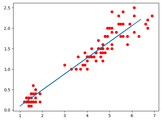
# 회귀분석 방법 4 - Elastic Net 회귀모형 : Ridge + Lasso
# 가중치 제곱합을 최소화, 거중치 절대값의 합을 최소화, 두가지를 동시에 제약조건으로 사용
from sklearn.linear_model import ElasticNet
'BACK END > Deep Learning' 카테고리의 다른 글
| [딥러닝] 로지스틱 회귀 (0) | 2021.03.15 |
|---|---|
| [딥러닝] 다항회귀 (0) | 2021.03.12 |
| [딥러닝] 선형회귀 (0) | 2021.03.10 |
| [딥러닝] 공분산, 상관계수 (0) | 2021.03.10 |
| [딥러닝] 이항검정 (0) | 2021.03.10 |