SVM(Support Vector Machine)
: 두 데이터 사이에 구분을 위해 사용
: 각 데이터의 중심을 기준으로 초평면(Optimal Hyper Plane) 구한다.
: 초평면과 가까운 데이터를 support vector라 한다.
: XOR 처리 가능
XOR 연산 처리(분류)
* svm1.py
xor_data = [
    [0,0,0],
    [0,1,1],
    [1,0,1],
    [1,1,0],
]
#print(xor_data)

import pandas as pd
import numpy as np
from sklearn.linear_model import LogisticRegression
from sklearn import svm

xor_df = pd.DataFrame(xor_data)

feature = np.array(xor_df.iloc[:, 0:2])
label = np.array(xor_df.iloc[:, 2])
print(feature)
'''
[[0 0]
 [0 1]
 [1 0]
 [1 1]]
'''
print(label) # [0 1 1 0]
model = LogisticRegression() # 선형분류 모델
model.fit(feature, label)
pred = model.predict(feature)
print('pred :', pred)
# pred : [0 0 0 0]
model = svm.SVC() # 선형, 비선형(kernel trick 사용) 분류모델
model.fit(feature, label)
pred = model.predict(feature)
print('pred :', pred)
# pred : [0 1 1 0]# Sopport vector 확인해보기
from sklearn.datasets import make_blobs
import matplotlib.pyplot as plt
import numpy as np
plt.rc('font', family='malgun gothic')
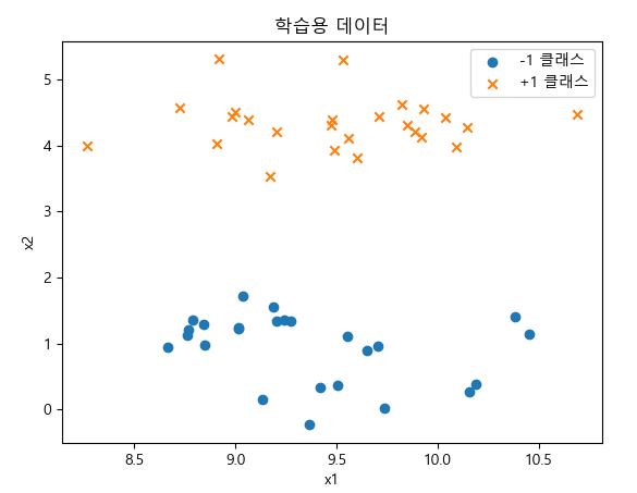
X, y = make_blobs(n_samples=50, centers=2, cluster_std=0.5, random_state=4)
y = 2 * y - 1
plt.scatter(X[y == -1, 0], X[y == -1, 1], marker='o', label="-1 클래스")
plt.scatter(X[y == +1, 0], X[y == +1, 1], marker='x', label="+1 클래스")
plt.xlabel("x1")
plt.ylabel("x2")
plt.legend()
plt.title("학습용 데이터")
plt.show()
from sklearn.svm import SVC
model = SVC(kernel='linear', C=1.0).fit(X, y) # tuning parameter 값을 변경해보자.
xmin = X[:, 0].min()
xmax = X[:, 0].max()
ymin = X[:, 1].min()
ymax = X[:, 1].max()
xx = np.linspace(xmin, xmax, 10)
yy = np.linspace(ymin, ymax, 10)
X1, X2 = np.meshgrid(xx, yy)
z = np.empty(X1.shape)
for (i, j), val in np.ndenumerate(X1): # 배열 좌표와 값 쌍을 생성하는 반복기를 반환
x1 = val
x2 = X2[i, j]
p = model.decision_function([[x1, x2]])
z[i, j] = p[0]
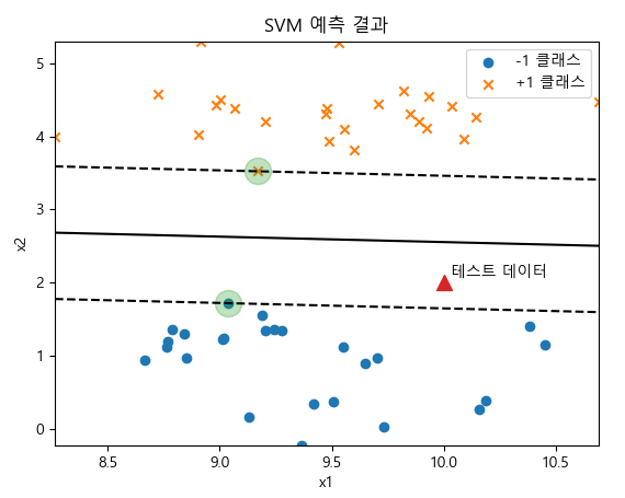
levels = [-1, 0, 1]
linestyles = ['dashed', 'solid', 'dashed']
plt.scatter(X[y == -1, 0], X[y == -1, 1], marker='o', label="-1 클래스")
plt.scatter(X[y == +1, 0], X[y == +1, 1], marker='x', label="+1 클래스")
plt.contour(X1, X2, z, levels, colors='k', linestyles=linestyles)
plt.scatter(model.support_vectors_[:, 0], model.support_vectors_[:, 1], s=300, alpha=0.3)
x_new = [10, 2]
plt.scatter(x_new[0], x_new[1], marker='^', s=100)
plt.text(x_new[0] + 0.03, x_new[1] + 0.08, "테스트 데이터")
plt.xlabel("x1")
plt.ylabel("x2")
plt.legend()
plt.title("SVM 예측 결과")
plt.show()
# Support Vectors 값 출력
print(model.support_vectors_)
'''
[[9.03715314 1.71813465]
[9.17124955 3.52485535]]
'''
* svm2_iris.py
BMI의 계산방법을 이용하여 많은 양의 자료를 생성한 후 분류 모델로 처리
계산식 신체질량지수(BMI)=체중(kg)/[신장(m)]2
판정기준 저체중 20 미만
정상 20 - 24
과체중 25 - 29
비만 30 이상
* svm3_bmi.py
print(67/((170 / 100) * (170 / 100)))

import random

def calc_bmi(h,w):
    bmi = w / (h / 100)**2
    if bmi < 18.5: return 'thin'
    if bmi < 23: return 'normal'
    return 'fat'
print(calc_bmi(170, 65))
fp = open('bmi.csv', 'w')
fp.write('height, weight, label\n')
cnt = {'thin':0, 'normal':0, 'fat':0}
for i in range(50000):
h = random.randint(150, 200)
w = random.randint(35, 100)
label = calc_bmi(h, w)
cnt[label] += 1
fp.write('{0},{1},{2}\n'.format(h, w, label))
fp.close()
print('good')# BMI dataset으로 분류
from sklearn import svm, metrics
from sklearn.model_selection import train_test_split
import pandas as pd
import matplotlib.pyplot as plt
tbl = pd.read_csv('bmi.csv')
# 칼럼을 정규화
label = tbl['label']
print(label)
w = tbl['weight'] / 100
h = tbl['height'] / 200
wh = pd.concat([w, h], axis=1)
print(wh.head(5), wh.shape)
'''
weight height
0 0.69 0.850
1 0.51 0.835
2 0.70 0.830
3 0.71 0.945
4 0.50 0.980 (50000, 2)
'''
label = label.map({'thin':0, 'normal':1, 'fat':2})
'''
0 2
1 0
2 2
3 1
4 0
'''
print(label[:5], label.shape) # (50000,)# train/test
data_train, data_test, label_train, label_test = train_test_split(wh, label)
print(data_train.shape, data_test.shape) # (37500, 2) (12500, 2)
# model
model = svm.SVC(C=0.01).fit(data_train, label_train)
#model = svm.LinearSVC().fit(data_train, label_train)
print(model)# 학습한 데이터의 결과가 신뢰성이 있는지 확인하기 위해 교차검증 p221
from sklearn import model_selection
cross_vali = model_selection.cross_val_score(model, wh, label, cv=3)
# k ford classification
# train 7, test 3 => train으로 3등분 하여 재검증
# 검증 학습 학습
# 학습 검증 학습
# 학습 학습 검증
print('각각의 검증 결과:', cross_vali) # [0.96754065 0.96400072 0.96783871]
print('평균 검증 결과:', cross_vali.mean()) # 0.9664600275737195pred = model.predict(data_test)
ac_score = metrics.accuracy_score(label_test, pred)
print('분류 정확도 :', ac_score) # 분류 정확도 : 0.96816
print(metrics.classification_report(label_test, pred))
'''
precision recall f1-score support
0 0.98 0.97 0.98 4263
1 0.91 0.94 0.93 2644
2 0.98 0.98 0.98 5593
accuracy 0.97 12500
macro avg 0.96 0.96 0.96 12500
weighted avg 0.97 0.97 0.97 12500
'''# 시각화
tbl2 = pd.read_csv('bmi.csv', index_col = 2)
print(tbl2[:3])
'''
height weight
label
fat 170 69
thin 167 51
fat 166 70
'''
def scatter_func(lbl, color):
b = tbl2.loc[lbl]
plt.scatter(b['weight'], b['height'], c=color, label=lbl)
fig = plt.figure()
scatter_func('fat', 'red')
scatter_func('normal', 'yellow')
scatter_func('thin', 'blue')
plt.legend()
plt.savefig('bmi_test.png')
plt.show()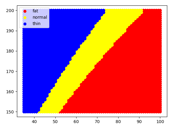
SVM 모델로 이미지 분류
* svm4.py
afrom sklearn.datasets import fetch_lfw_people
fetch_lfw_people(min_faces_per_person = 60) : 인물 사진 data load. min_faces_per_person : 최초
scikit-learn.org/stable/modules/generated/sklearn.datasets.fetch_lfw_people.html
sklearn.datasets.fetch_lfw_people — scikit-learn 0.24.1 documentation
scikit-learn.org
import matplotlib.pyplot as plt
from sklearn.metrics._classification import classification_report

faces = fetch_lfw_people(min_faces_per_person = 60)
print(faces)

print(faces.DESCR)
print(faces.data)
print(faces.data.shape) # (729, 2914)
print(faces.target)
print(faces.target_names)
print(faces.images.shape) # (729, 62, 47)

print(faces.images[0])
print(faces.target_names[faces.target[0]])
plt.imshow(faces.images[0], cmap='bone') # cmap : 색
plt.show()

fig, ax = plt.subplots(3, 5)
print(fig)          # Figure(640x480)
print(ax.flat)      # <numpy.flatiter object at 0x00000235198C5D30>
print(len(ax.flat)) # 15
for i, axi in enumerate(ax.flat):
    axi.imshow(faces.images[i], cmap='bone')
    axi.set(xticks=[], yticks=[], xlabel=faces.target_names[faces.target[i]])
plt.show()
- 주성분 분석으로 이미지 차원을 축소시켜 분류작업을 진행
from sklearn.svm import SVC
from sklearn.decomposition import PCA
from sklearn.pipeline import make_pipeline

m_pca = PCA(n_components=150, whiten=True, random_state = 0)
m_svc = SVC(C=1)
model = make_pipeline(m_pca, m_svc)
print(model)
# Pipeline(steps=[('pca', PCA(n_components=150, random_state=0, whiten=True)),
#                 ('svc', SVC(C=1))])
- train/test
from sklearn.model_selection import train_test_split

x_train, x_test, y_train, y_test = train_test_split(faces.data, faces.target, random_state=1)
print(x_train[0], x_train.shape) # (546, 2914)
print(y_train[0], y_train.shape) # (546,)

model.fit(x_train, y_train)  # train data로 모델 fitting
pred = model.predict(x_test)
print('pred :', pred)   # pred : [1 1 1 1 1 1 1 1 1 1 1 0 1 1 1 ..
print('read :', y_test) # read : [0 1 1 1 1 1 1 1 1 1 1 0 1 1 1 ..
- 분류 정확도
from sklearn.metrics import classification_report

print(classification_report(y_test, pred, target_names = faces.target_names)) # 분류 정확도
'''
                   precision    recall  f1-score   support

  Donald Rumsfeld       1.00      0.25      0.40        20
    George W Bush       0.80      1.00      0.89       132
Gerhard Schroeder       1.00      0.45      0.62        31

         accuracy                           0.83       183
        macro avg       0.93      0.57      0.64       183
     weighted avg       0.86      0.83      0.79       183
=> f1-score/accuracy -> 0.83
'''

from sklearn.metrics import confusion_matrix, accuracy_score

mat = confusion_matrix(y_test, pred)
print('confusion_matrix :\n', mat)
'''
 [[  5  15   0]
 [  0 132   0]
 [  0  17  14]]
 '''
print('acc :', accuracy_score(y_test, pred)) # 0.82513
- 분류결과를 시각화
# x_test[0] 하나 미리보기.
plt.subplots(1, 1)
print(x_test[0], ' ', x_test[0].shape)
# [ 24.333334  33.        72.666664 ... 201.66667  201.33333  155.33333 ]   (2914,)
print(x_test[0].reshape(62, 47)) # 1차원을 2차원으로 변환해야 이미지 출력 가능
plt.imshow(x_test[0].reshape(62, 47), cmap='bone')
plt.show()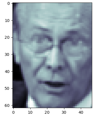
fig, ax = plt.subplots(4, 6)
for i, axi in enumerate(ax.flat):
    axi.imshow(x_test[i].reshape(62, 47), cmap='bone')
    axi.set(xticks=[], yticks=[])
    axi.set_ylabel(faces.target_names[pred[i]].split()[-1], color='black' if pred[i] == y_test[i] else 'red')
    fig.suptitle('pred result', size = 14)
plt.show()
- 5차 행렬 시각화
import seaborn as sns
sns.heatmap(mat.T, square = True, annot=True, fmt='d', cbar=False, \
            xticklabels=faces.target_names, yticklabels=faces.target_names)
plt.xlabel('true(read) label')
plt.ylabel('predicted label')
plt.show()

'BACK END > Deep Learning' 카테고리의 다른 글
| [딥러닝] 나이브 베이즈 (0) | 2021.03.17 |
|---|---|
| [딥러닝] PCA (0) | 2021.03.16 |
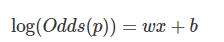
| [딥러닝] 로지스틱 회귀 (0) | 2021.03.15 |
| [딥러닝] 다항회귀 (0) | 2021.03.12 |
| [딥러닝] 단순선형 회귀, 다중선형 회귀 (0) | 2021.03.11 |