21. 군집분석(Clustering) : 비지도학습 - 유클리디안 거리 계산법 사용
x <- matrix(1:16, nrow = 4)
x
# [,1] [,2] [,3] [,4]
# [1,]    1    5    9   13
# [2,]    2    6   10   14
# [3,]    3    7   11   15
# [4,]    4    8   12   16
help(dist)
d <- dist(x, method = "euclidean")
d
#   1 2 3
# 2 2
# 3 4 2
# 4 6 4 2
plot(d)
text(d, c(LETTERS[1:6]))
txt1 <- read.csv("testdata/cluster_ex.csv")
txt1
# irum kor eng
# 1 홍길동  80  90
# 2 이기자  70  40
# 3 유별나  65  75
# 4 강나루  85  65
# 5 전속력  95  87
plot(txt1[, c(2:3)],
     xlab ='국어',
     ylab ='영어',
     xlim = c(30, 100),
     ylim = c(30, 100),
     main = '학생점수')

text(txt1[, 2], txt1[, 3], labels = abbreviate(rownames(txt1)), cex = 0.8, pos = 1, col = "blue")
text(txt1[, 2], txt1[, 3], labels = txt1[,1], cex = 0.8, pos = 2, col = "red")
dist_m <- dist(txt1[c(1:2), c(2:3)], method = "manhattan")
dist_m
# 1
# 2 60

dist_e <- dist(txt1[c(1:2), c(2:3)], method = "euclidean")
dist_e
# 1
# 2 50.9902
- 계층적 군집분석
x <- c(1,2,2,4,5)
y <- c(1,1,4,3,5)
xy <- data.frame(cbind(x,y))
plot(xy,
     xlab ='x',
     ylab ='y',
     xlim = c(0, 6),
     ylim = c(0, 6),
     main = '응집적 군집분석')

text(xy[, 1], xy[, 2], labels = abbreviate(rownames(xy)),
     cex = 0.8, pos = 1, col = "blue")
abline(v=c(3), col = 'gray', lty=2)
abline(h=c(3), col = 'gray', lty=2)

- 유클리디안 거리 계산법
dist(xy, method = 'euclidean') ^ 2
#    1  2  3  4
# 2  1
# 3 10  9
# 4 13  8  5
# 5 32 25 10  5
- Dendrogram으로 출력
hc_sl <- hclust(dist(xy) ^ 2, method = "single") # 최단거리법
hc_sl
plot(hc_sl, hang = -1)

hc_co <- hclust(dist(xy) ^ 2, method = "complete") # 완전(최장) 거리법
hc_co
plot(hc_co, hang = -1)

hc_av <- hclust(dist(xy) ^ 2, method = "average") # 평균 거리법
hc_av
plot(hc_av, hang = -1)

par(oma = c(3, 0, 1, 0))
par(mfrow = c(1,3))
plot(hc_sl, hang = -1)
plot(hc_co, hang = -1)
plot(hc_av, hang = -1)
- 중학생 신체검사 결과
body <- read.csv("testdata/bodycheck.csv")
body
#      번호 악력 신장 체중 안경유무
# 1     1   28  146   34        1
# 2     2   46  169   57        2
# 3     3   39  160   48        2
# 4     4   25  156   38        1
# 5     5   34  161   47        1
# 6     6   29  168   50        1
# 7     7   38  154   54        2
# 8     8   23  153   40        1
# 9     9   42  160   62        2
# 10   10   27  152   39        1
# 11   11   35  155   46        1
# 12   12   39  154   54        2
# 13   13   38  157   57        2
# 14   14   32  162   53        2
# 15   15   25  142   32        1
dim(body)
head(body, 2)

d <- dist(body[, -1]) # 거리계산
d

hc <- hclust(d, method = "complete")
hc
# Cluster method   : complete
# Distance         : euclidean
# Number of objects: 15

plot(hc, hang=-1) # hang=-1 정렬
rect.hclust(hc, k=3, border = "red")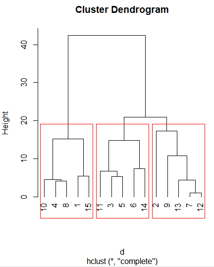
- 군집별 특징
g1 <- subset(body, 번호 == 10 |번호 == 4 |번호 == 8 |번호 == 1 |번호 == 15)
g2 <- subset(body, 번호 == 11 |번호 == 3 |번호 == 5 |번호 == 6 |번호 == 14)
g3 <- subset(body, 번호 == 2 |번호 == 9 |번호 == 13 |번호 == 7 |번호 == 12)

g1[2:5]
g2[2:5]
g3[2:5]

summary(g1[2:5])
summary(g2[2:5])
summary(g3[2:5])'BACK END > R' 카테고리의 다른 글
| [R] R 정리 23 - 비계층적 군집분석2 (k-means) (0) | 2021.02.05 |
|---|---|
| [R] R 정리 22 - 비계층적 군집분석 (0) | 2021.02.04 |
| [R] R 정리 20 - MLP(deep learning) (0) | 2021.02.04 |
| [R] R 정리 19 - ANN(인공 신경망) (0) | 2021.02.03 |
| [R] R 정리 18 - svm, knn (0) | 2021.02.02 |