mglearn.discrete_scatter(X[:, 0], X[:, 1], y, ax=ax)
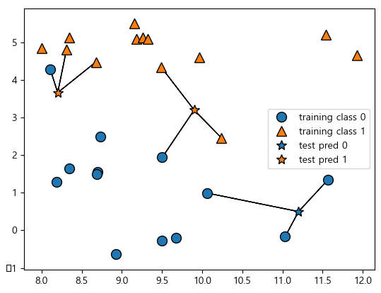
왼쪽 그림을 보면 이웃을 하나 선택했을 때는 결정 경계가 훈련 데이터에 가깝게 따라가고 있습니다. 이웃의 수를 늘릴수록 결정 경계는 더 부드러워집니다. 부드러운 경계는 더 단순한 모델을 의미합니다. 다시 말해 이웃을 적게 사용하면 모델의 복잡도가 높아지고([그림]의 오른쪽) 많이 사용하면 복잡도는 낮아집니다([그림]의 왼쪽).
훈련 데이터 전체 개수를 이웃의 수로 지정하는 극단적인 경우에는 모든 테스트 포인트가 같은 이웃(모든 훈련 데이터)을 가지게 되므로 테스트 포인트에 대한 예측은 모두 같은 값이 됩니다. 즉 훈련 세트에서 가장 많은 데이터 포인트를 가진 클래스가 예측값이 됩니다. 일반적으로 KNeighbors 분류기에 중요한 매개변수는 두 개입니다. 데이터 포인트 사이의 거리를 재는 방법과 이웃의 수입니다. 실제로 이웃의 수는 3개나 5개 정도로 적을 때 잘 작동하지만, 이 매개변수는 잘 조정해야 합니다. 거리 재는 방법은 기본적으로 유클리디안 거리 방식을 사용합니다.
breast_cancer dataset으로 실습
from sklearn.datasets import load_breast_cancer

cancer = load_breast_cancer()
X_train, X_test, y_train, y_test = train_test_split(cancer.data, cancer.target, stratify=cancer.target, random_state=66)

training_accuracy = []
test_accuracy = []
# 1에서 10까지 n_neighbors를 적용
neighbors_settings = range(1, 11)

for n_neighbors in neighbors_settings:
    clf = KNeighborsClassifier(n_neighbors=n_neighbors)  # 모델 생성
    clf.fit(X_train, y_train)
    # train dataset 정확도 저장
    training_accuracy.append(clf.score(X_train, y_train))
    # test dataset 정확도 저장
    test_accuracy.append(clf.score(X_test, y_test))

import numpy as np
print("평균 정확도 :", np.mean(test_accuracy))
# 평균 정확도 : 0.918881118881119
plt.plot(neighbors_settings, training_accuracy, label="훈련 정확도")
plt.plot(neighbors_settings, test_accuracy, label="테스트 정확도")
plt.ylabel("정확도")
plt.xlabel("n_neighbors")
plt.legend()
plt.show()
from sklearn.datasets import load_breast_cancer load_breast_cancer()
이 그림은 n_neighbors 수(x축)에 따른 훈련 세트와 테스트 세트 정확도(y축)를 보여줍니다. 실제 이런 그래프는 매끈하게 나오지 않지만, 여기서도 과대적합과 과소적합의 특징을 볼 수 있습니다 (이웃의 수가 적을수록 모델이 복잡해지므로 [그림]의 그래프가 수평으로 뒤집힌 형태입니다). 최근접 이웃의 수가 하나일 때는 훈련 데이터에 대한 예측이 완벽합니다. 하지만 이웃의 수가 늘어나면 모델은 단순해지고 훈련 데이터의 정확도는 줄어듭니다. 이웃을 하나 사용한 테스트 세트의 정확도는 이웃을 많이 사용했을 때보다 낮습니다. 이것은 1-최근접 이웃이 모델을 너무 복잡하게 만든다는 것을 설명해줍니다. 반대로 이웃을 10개 사용했을 때는 모델이 너무 단순해서 정확도는 더 나빠집니다. 정확도가 가장 좋을 때는 중간 정도인 여섯 개를 사용한 경우입니다.
참고 : 파이썬 라이브러리를 활용한 머신러닝 (한빛미디어 출판사)의 일부분을 사용했습니다.
pd.set_option('display.max_columns', 100) # 데이터 프레임 출력시 생략 값 출력.
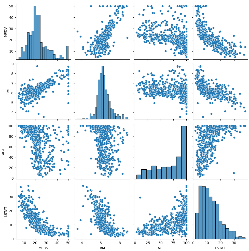
print(df.corr()) # 상관계수 확인
# RM average number of rooms per dwelling. 상관계수 : 0.695360
# AGE proportion of owner-occupied units built prior to 1940. 상관계수 : -0.376955
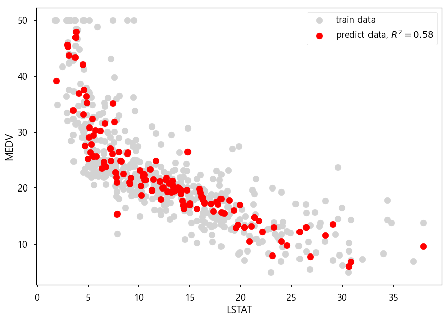
# LSTAT % lower status of the population 상관계수 : -0.737663
배깅(Bagging) - Random Forest : 데이터에서 여러 bootstrap 자료 생성, 모델링 후 결합하여 최종 예측 모형을 만드는 알고리즘 boostrap aggregating의 약어로 데이터를 가방(bag)에 쓸어 담아 복원 추출하여 여러 개의 표본을 만들어 이를 기반으로 각각의 모델을 개발한 후에 결과를 하나로 합쳐 하나의 모델을 만들어 내는 것이다. 배깅을 통해서 얻을 수 있는 효과는 '알고리즘의 안정성'이다. 단일 seed 하나의 값을 기준으로 데이터를 추출하여 모델을 생성해 나는 것보다, 여러 개의 다양한 표본을 사용함으로써 모델을 만드는 것이 모집단을 잘 대표할 수 있게 된다. 또한 명목형 변수 (Categorical data)의 경우 투표(voting) 방식, 혹은 가장 높은 확률값으로 예측 결과값을 합치며 연속형 변수(numeric data)의 경우에는 평균(average)으로 값을 집계한다. 또한 배깅은 병렬 처리를 사용할 수 있는데, 독립적인 데이터 셋으로 독립된 모델을 만들기 때문에 모델 생성에 있어서 매우 효율적이다.
부스팅(Boosting) - XGBoost : 오분류 개체들에 가중치를 적용하여 새로운 분류 규칙 생성 반복 기반 최종 예측 모형 생성 좀 더 알아보자면 Boosting이란 약한 분류기를 결합하여 강한 분류기를 만드는 과정이다. 분류기 A, B, C 가 있고, 각각의 0.3 정도의 accuracy를 보여준다고 하자. A, B, C를 결합하여 더 높은 정확도, 예를 들어 0.7 정도의 accuracy를 얻는 게 앙상블 알고리즘의 기본 원리다. Boosting은 이 과정을 순차적으로 실행한다. A 분류기를 만든 후, 그 정보를 바탕으로 B 분류기를 만들고, 다시 그 정보를 바탕으로 C 분류기를 만든다. 그리고 최종적으로 만들어진 분류기들을 모두 결합하여 최종 모델을 만드는 것이 Boosting의 원리다. 대표적인 알고리즘으로 에이다부스트가 있다. AdaBoost는 Adaptive Boosting의 약자이다. Adaboost는 ensemble-based classifier의 일종으로 weak classifier를 반복적으로 적용해서, data의 특징을 찾아가는 알고리즘.
- anaconda prompt
pip install xgboost
*xgboost1.py
# RandomForest vs xgboost
import pandas as pd
from sklearn import datasets
from sklearn.model_selection import train_test_split
from sklearn.ensemble import RandomForestClassifier
from sklearn import metrics
import numpy as np
import xgboost as xgb       # pip install xgboost

if __name__ == '__main__':
    iris = datasets.load_iris()
    print('아이리스 종류 :', iris.target_names)
    print('데이터 열 이름 :', iris.feature_names)

    # iris data로 Dataframe
    data = pd.DataFrame(
        {
            'sepal length': iris.data[:, 0],
            'sepal width': iris.data[:, 1],
            'petal length': iris.data[:, 2],
            'petal width': iris.data[:, 3],
            'species': iris.target
        }
    )
    print(data.head(2))
    '''
           sepal length  sepal width  petal length  petal width  species
    0           5.1          3.5           1.4          0.2        0
    1           4.9          3.0           1.4          0.2        0
    '''

    x = data[['sepal length', 'sepal width', 'petal length', 'petal width']]
    y = data['species']

    # 테스트 데이터 30%
    x_train, x_test, y_train, y_test = train_test_split(x, y, test_size=0.3, random_state=123)

    # 학습 진행
    model = RandomForestClassifier(n_estimators=100)  # RandomForestClassifier - Bagging 방법 : 병렬 처리
    model = xgb.XGBClassifier(booster='gbtree', max_depth=4, n_estimators=100) # XGBClassifier - Boosting : 직렬처리
    # 속성 - booster: 의사결정 기반 모형(gbtree), 선형 모형(linear)
    #    - max_depth [기본값: 6]: 과적합 방지를 위해서 사용되며 CV를 사용해서 적절한 값이 제시되어야 하고 보통 3-10 사이 값이 적용된다.

    model.fit(x_train, y_train)

    # 예측
    y_pred = model.predict(x_test)
    print('예측값 : ', y_pred[:5])
    # 예측값 :  [1 2 2 1 0]

    print('실제값 : ', np.array(y_test[:5]))
    # 실제값 :  [1 2 2 1 0]

    print('정확도 : ', metrics.accuracy_score(y_test, y_pred))
    # 정확도 :  0.9333333333333333
import xgboost as xgb
xgb.XGBClassifier(booster='gbtree', max_depth=, n_estimators=) : XGBoost 분류 - Boosting(직렬처리) booster : 의사결정 기반 모형(gbtree), 선형 모형(linear) max_depth : 과적합 방지를 위해서 사용되며 CV를 사용해서 적절한 값이 제시되어야 하고 보통 3-10 사이 값이 적용됨.
# 시각화 - graphviz 툴을 사용
import collections

dot_data = tree.export_graphviz(model, feature_names=label_names, out_file=None,\
                                filled = True, rounded=True)
graph = pydotplus.graph_from_dot_data(dot_data)
colors = ('red', 'orange')
edges = collections.defaultdict(list) # list type 변수

for e in graph.get_edge_list():
    edges[e.get_source()].append(int(e.get_destination()))

for e in edges:
    edges[e].sort()
    for i in range(2):
        dest = graph.get_node(str(edges[e][i]))[0]
        dest.set_fillcolor(colors[i])

graph.write_png('tree.png') # 이미지 저장

import matplotlib.pyplot as plt

img = plt.imread('tree.png')
plt.imshow(img)
plt.show()
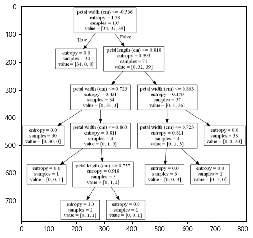
* tree2_iris.py
...

# 의사결정 나무 모델
from sklearn.tree import DecisionTreeClassifier
model = DecisionTreeClassifier(criterion='entropy', max_depth=5)

...
...
# 트리의 특성 중요도 : 전체 트리 결정에 각 특성이 어느정도 중요한지 평가
print('특성 중요도 : \n{}'.format(model.feature_importances_))

def plot_feature_importances(model):
    n_features = x.shape[1] # 4
    plt.barh(range(n_features), model.feature_importances_, align='center')
    #plt.yticks(np.range(n_features), iris.featrue_names[2:4])
    plt.xlabel('특성중요도')
    plt.ylabel('특성')
    plt.ylim(-1, n_features)

plot_feature_importances(model)
plt.show()
# graphviz
from sklearn import tree
from io import StringIO
import pydotplus

dot_data = StringIO() # 파일 흉내를 내는 역할
tree.export_graphviz(model, out_file = dot_data,\
                     feature_names = iris.feature_names[2:4])
graph = pydotplus.graph_from_dot_data(dot_data.getvalue())
graph.write_png('tree2.png')

import matplotlib.pyplot as plt

img = plt.imread('tree2.png')
plt.imshow(img)
plt.show()
from sklearn.preprocessing import OneHotEncoder
x = '1,2,3,4,5'
x = x.split(',')
x = np.array(x)
x = x[:, np.newaxis]
'''
[['1']
 ['2']
 ['3']
 ['4']
 ['5']]
'''

one_hot = OneHotEncoder(categories = 'auto')
x = one_hot.fit_transform(x).toarray()
print(x)
'''
[[1. 0. 0. 0. 0.]
 [0. 1. 0. 0. 0.]
 [0. 0. 1. 0. 0.]
 [0. 0. 0. 1. 0.]
 [0. 0. 0. 0. 1.]]
'''
y = np.array([1,3,5,7,9])

model = GaussianNB().fit(x, y)
pred = model.predict(x)
print(pred) # [1 3 5 7 9]
print('acc :', metrics.accuracy_score(y, pred)) # acc : 1.0
* bayes3_text.py
# 나이브베이즈 분류모델로 텍스트 분류
from sklearn.datasets import fetch_20newsgroups

data = fetch_20newsgroups()
print(data.target_names)

categories = ['talk.religion.misc', 'soc.religion.christian',
              'sci.space', 'comp.graphics']

train = fetch_20newsgroups(subset='train', categories=categories)
test = fetch_20newsgroups(subset='test', categories=categories)
print(train.data[5])  # 데이터 중 대표항목

from sklearn.feature_extraction.text import TfidfVectorizer
from sklearn.naive_bayes import MultinomialNB
from sklearn.pipeline import make_pipeline

# 각 문자열의 콘텐츠를 숫자벡터로 전환
model = make_pipeline(TfidfVectorizer(), MultinomialNB())  # 작업을 연속적으로 진행
model.fit(train.data, train.target)
labels = model.predict(test.data)

from sklearn.metrics import confusion_matrix
import matplotlib.pyplot as plt
import seaborn as sns

mat = confusion_matrix(test.target, labels)  # 오차행렬 보기
sns.heatmap(mat.T, square=True, annot=True, fmt='d', cbar=False,
            xticklabels=train.target_names, yticklabels=train.target_names)
plt.xlabel('true label')
plt.ylabel('predicted label')
plt.show()

# 하나의 문자열에 대해 예측한 범주 변환용 유틸 함수 작성
def predict_category(s, train=train, model=model):
    pred = model.predict([s])
    return train.target_names[pred[0]]

print(predict_category('sending a payload to the ISS'))
print(predict_category('discussing islam vs atheism'))
print(predict_category('determining the screen resolution'))

# 참고 도서 : 파이썬 데이터사이언스 핸드북 ( 출판사 : 위키북스)
# 학습한 데이터의 결과가 신뢰성이 있는지 확인하기 위해 교차검증 p221
from sklearn import model_selection
cross_vali = model_selection.cross_val_score(model, wh, label, cv=3)
# k ford classification
# train 7, test 3 => train으로 3등분 하여 재검증
# 검증 학습 학습
# 학습 검증 학습
# 학습 학습 검증
print('각각의 검증 결과:', cross_vali)          # [0.96754065 0.96400072 0.96783871]
print('평균 검증 결과:', cross_vali.mean())    # 0.9664600275737195
- 출력된 연속형 자료에 대해 odds -> odds ratio -> logit function -> sigmoid function으로 이항분류
- odds(오즈)
: 확률을 바꾼 값. 성공확률(혹은 1일)이 실패확률(0일)에 비해 몇 배 더 높은가를 나타낸다.
- odds ratio(오즈비)
: 두 개의 오즈 비율. 확률 p의 범위가 (0,1)이라면 Odds(p)의 범위는 (0, ∞)이 된다.
- logit(로짓)
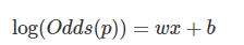
: 오즈비에 로그를 취한 값. Odds ratio에 로그함수를 취한 log(Odds(p))은 입력값의 범위가 (-∞ ~ ∞)이 된다. 즉, 범위가 실수 전체다. 이러한 입력 값의 범위를 (0 ~ 1)로 조정한다.
- sigmoid(시그모이드)
: log(Odds(p))의 범위가 실수이므로 이 값에 대한 선형회귀분석을 하는 것은 의미가 있다. 왜냐하면 오즈비(두 개의 odd 비율)에 로그를 씌우면 오즈비 값들이 정규분포를 이루기 때문이다. log(Odds(p))=wx+b로 선형회귀분석을 실시해서 w와 b를 얻을 수 있다. 위 식을 이용한 것이 sigmoid function이다. 이를 통해 0.5을 기준으로 1과 0의 양분된 값을 된다.
print('추정치 구하기 차체 무게를 입력해 연비를 추정')
result3 = smf.ols('mpg ~ wt', data=mtcars).fit()
print(result3.summary())
print('결정계수 :', result3.rsquared) # 0.7528327936582646 > 0.05 설명력이 우수한 모델
pred = result3.predict()
# 1개의 자료로 실제값과 예측값(추정값) 저장 후 비교
print(mtcars.mpg[0])
print(pred[0]) # 모든 자동차 차체 무게에 대한 연비 추정치 출력

data = {
    'mpg':mtcars.mpg,
    'mpg_pred':pred
    }
df = pd.DataFrame(data)
print(df)
'''
                      mpg   mpg_pred
Mazda RX4            21.0  23.282611
Mazda RX4 Wag        21.0  21.919770
Datsun 710           22.8  24.885952
'''
# 새로운 차체 무게로 연비 추정하기
mtcars.wt = float(input('차체 무게 입력:'))
new_pred = result3.predict(pd.DataFrame(mtcars.wt))
print('차체 무게 {}일때 예상연비{}이다'.format(mtcars.wt[0], new_pred[0]))
# 차체 무게 1일때 예상연비31.940654594619367이다
print('\n다중 선형회귀 모델 ')
lm_mul = smf.ols(formula = 'sales ~ tv + radio + newspaper', data = adf_df).fit()
#  + newspaper 포함시와 미포함시의 R2값 변화가 없어 제거 필요.
print(lm_mul.summary())
print(adf_df.corr())

# 예측2 : 새로운 tv, radio값으로 sales를 추정
x_new2 = pd.DataFrame({'tv':[230.1, 44.5, 100], 'radio':[30.1, 40.1, 50.1],\
                      'newspaper':[10.1, 10.1, 10.1]})
pred2 = lm.predict(x_new2)
print('추정값 :\n', pred2)
'''
0    17.970775
1     9.147974
2    11.786258
'''
회귀분석모형의 적절성을 위한 조건
: 아래의 조건 위배 시에는 변수 제거나 조정을 신중히 고려해야 함.
- 정규성 : 독립변수들의 잔차항이 정규분포를 따라야 한다. - 독립성 : 독립변수들 간의 값이 서로 관련성이 없어야 한다. - 선형성 : 독립변수의 변화에 따라 종속변수도 변화하나 일정한 패턴을 가지면 좋지 않다. - 등분산성 : 독립변수들의 오차(잔차)의 분산은 일정해야 한다. 특정한 패턴 없이 고르게 분포되어야 한다. - 다중공선성 : 독립변수들 간에 강한 상관관계로 인한 문제가 발생하지 않아야 한다.