[코딩] Circle Square

# SVM 분류 모델 : 데이터 분류 결정 마진에 영향을 주는 관측치(Support Vectors)를 이용
# Kernel trick을 이용해 비선형 데이터에 대한 분류도 가능

library(e1071)

# train/test 생략
head(iris, 3)
# Sepal.Length Sepal.Width Petal.Length Petal.Width Species
# 1          5.1         3.5          1.4         0.2  setosa
# 2          4.9         3.0          1.4         0.2  setosa
# 3          4.7         3.2          1.3         0.2  setosa
x <- subset(iris, select = -Species)
y <- iris$Species
x
y

svm_model <- svm(Species ~ ., data=iris)
svm_model
# Parameters:
#   SVM-Type:  C-classification 
# SVM-Kernel:  radial 
# cost:  1 
# 
# Number of Support Vectors:  51
summary(svm_model)

svm_model1 <- svm(x, y)
summary(svm_model1)

dist(iris[, -5])
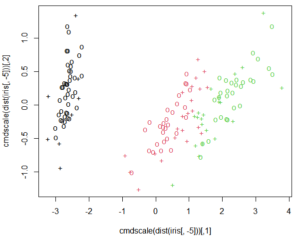
cmdscale(dist(iris[, -5])) # 거리 값을 공간적인 배치형식으로 출력
# [,1]         [,2]
# [1,] -2.684125626  0.319397247
# [2,] -2.714141687 -0.177001225
# [3,] -2.888990569 -0.144949426
# [4,] -2.745342856 -0.318298979
# [5,] -2.728716537  0.326754513
# [6,] -2.280859633  0.741330449
# [7,] -2.820537751 -0.089461385
# [8,] -2.626144973  0.163384960

# support vector : + , 나머지 데이터는 o
plot(cmdscale(dist(iris[, -5])), col=as.integer(iris[,5]), pch=c("o","+")[1:150 %in% svm_model$index + 1])

pred <- predict(svm_model, x)
head(pred)
t <- table(pred, y)
t
# y
# pred         setosa versicolor virginica
# setosa         50          0         0
# versicolor      0         48         2
# virginica       0          2        48
sum(diag(t)) / nrow(x) # 분류 정확도 : 0.9733333

# 최상의 모델을 만들기 위해 파라미터 조절 - svm 튜닝

svm_tune <- tune(svm, train.x = x, train.y = y, kernel='radial',
                 ranges = list(cost=10^(-1:2)), gamma=2^(-2:2))
                # 10-fold cross validation : 교차 검정
svm_tune
# - sampling method: 10-fold cross validation 
# 
# - best parameters:
#   cost
# 1
# 
# - best performance: 0.03333333 

svm_model_after_tune <- svm(Species ~ ., data=iris, kernel='radial', cost=1, gamma=0.5)
summary(svm_model_after_tune)

pred <- predict(svm_model_after_tune, x)
t <- table(pred, y)
t
# y
# pred         setosa versicolor virginica
# setosa         50          0         0
# versicolor      0         48         2
# virginica       0          2        48
sum(diag(t)) / nrow(x) # 0.9733333

# KNN : 최근접 이웃 알고리즘을 사용. k개의 원 안에 데이터 수 
# 또는 거리(유클디안 거리 계산법)에 의해 새로운 데이터를 분류.
# 비모수적 검정 분류 모형

install.packages("ggvis")
library(ggvis)

head(iris, 2)
iris %>% ggvis(~Petal.Length, ~Petal.Width, fill=~factor(Species))

# 분류 모델 중 Naive Bayes claaifier 모델 : 조건부 확률을 이용. P(A|B): 사건 A가 발생했을때 B가 발생할 확률

library(e1071) # Naive Bayes

set.seed(123)
ind <- sample(1:nrow(iris), nrow(iris) * 0.7, replace = FALSE)
train <- iris[ind, ]
test <- iris[-ind, ]

help(naiveBayes)
model <- naiveBayes(Species ~ ., data = train)
model
# naiveBayes.default(x = X, y = Y, laplace = laplace)
# 
# A-priori probabilities:
#   Y
# setosa versicolor  virginica 
# 0.3428571  0.3047619  0.3523810 
# 
# Conditional probabilities:
#   Sepal.Length
# Y                [,1]      [,2]
# setosa     4.966667 0.3741657
# versicolor 5.971875 0.4887340
# virginica  6.586486 0.7165357
# 
# Sepal.Width
# Y                [,1]      [,2]
# setosa     3.394444 0.4049299
# versicolor 2.787500 0.3250310
# virginica  2.948649 0.3500965
# 
# Petal.Length
# Y                [,1]      [,2]
# setosa     1.461111 0.1777282
# versicolor 4.309375 0.4423977
# virginica  5.529730 0.6235494
# 
# Petal.Width
# Y                 [,1]      [,2]
# setosa     0.2555556 0.1157447
# versicolor 1.3500000 0.1951013
# virginica  1.9945946 0.2613490

pred <- predict(model, test, type='class')
head(pred, 3)
t <- table(pred, test$Species)
t
# pred         setosa versicolor virginica
# setosa         14          0         0
# versicolor      0         18         0
# virginica       0          0        13
sum(diag(t)) / nrow(test) # 1

prop.table(t) # margin = 1
# pred             setosa versicolor  virginica
# setosa     0.33333333 0.00000000 0.00000000
# versicolor 0.00000000 0.37777778 0.02222222
# virginica  0.00000000 0.00000000 0.26666667

#Random Forest 분류 모델 나무 구조 모델을 여러 개 합칩 모델(앙상블 기법)

install.packages("randomForest")
library(randomForest)

set.seed(123)
ind <- sample(1:nrow(iris), nrow(iris) * 0.7, replace = FALSE)
train <- iris[ind, ]
test <- iris[-ind, ]

model <- randomForest(formula=Species ~ ., data=train)
model
# randomForest(formula = Species ~ ., data = train) 
# Type of random forest: classification
# Number of trees: 500
# No. of variables tried at each split: 2
# 
# OOB estimate of  error rate: 5.71%
# Confusion matrix:
#   setosa versicolor virginica class.error
# setosa         36          0         0  0.00000000
# versicolor      0         29         3  0.09375000
# virginica       0          3        34  0.08108108

model2 <- randomForest(formula=Species ~ ., data=train, ntree = 200, mtry = 3, na.action = na.omit)
model2
# randomForest(formula = Species ~ ., data = train, ntree = 200,      mtry = 3, na.action = na.omit) 
# Type of random forest: classification
# Number of trees: 200
# No. of variables tried at each split: 3
# 
# OOB estimate of  error rate: 4.76%
# Confusion matrix:
#   setosa versicolor virginica class.error
# setosa         36          0         0  0.00000000
# versicolor      0         30         2  0.06250000
# virginica       0          3        34  0.08108108

model3 <- randomForest(formula=Species ~ ., data=train, ntree = 1000, mtry = 2, na.action = na.omit)
model3

# 모델 성능 향상을 위한 변수 선택, ntree, mtry 설정하기
# 중요 변수

model4 <- randomForest(Species ~ ., data=train, importance = T)
importance(model4) # Petal.Width가 가장 중요한 변수
# setosa versicolor virginica MeanDecreaseAccuracy MeanDecreaseGini
# Sepal.Length  5.947974  9.6040622  7.628999            12.547747         6.743408
# Sepal.Width   4.143228 -0.5277106  7.616918             6.344268         1.895498
# Petal.Length 22.586135 31.0203420 28.842917            34.060288        30.182599
# Petal.Width  21.470279 27.2038165 30.353685            32.467796        30.336028

varImpPlot(model4)

#pred

pred <- predict(model, test)
pred
t <- table(pred, test$Species)
t
# pred         setosa versicolor virginica
# setosa         14          0         0
# versicolor      0         17         0
# virginica       0          1        13

sum(diag(t)) / nrow(test) # 0.9777778

#..
pred4 <- predict(model4, test)
pred4
t4 <- table(pred4, test$Species)
sum(diag(t4)) / nrow(test) # 0.9777778

# ntree, mtry 최적 값 얻기

ntree <- c(400, 500, 600)
mtry <- c(2:4)
param <- data.frame(n=ntree, m=mtry)

for(i in param$n){
  cat('ntree : ', i, '\n')
  for(j in param$m){
    cat('mtree : ', j, '\n')
    model_ir = randomForest(Species ~ ., data=iris, ntree=i, mtry=j, na.action = na.omit)
    print(model_ir)
  }
}

# 분류모델 중 Decision Tree

set.seed(123)
ind <- sample(1:nrow(iris), nrow(iris) * 0.7, replace = FALSE)
train <- iris[ind, ]
test <- iris[-ind, ]

# ctree

install.packages("party")
library(party)
iris_ctree <- ctree(formula = Species ~ ., data = train)
iris_ctree
# Conditional inference tree with 4 terminal nodes
# 
# Response:  Species 
# Inputs:  Sepal.Length, Sepal.Width, Petal.Length, Petal.Width 
# Number of observations:  105 
# 
# 1) Petal.Length <= 1.9; criterion = 1, statistic = 97.466
# 2)*  weights = 36 
# 1) Petal.Length > 1.9
# 3) Petal.Width <= 1.7; criterion = 1, statistic = 45.022
# 4) Petal.Length <= 4.6; criterion = 0.987, statistic = 8.721
# 5)*  weights = 25 
# 4) Petal.Length > 4.6
# 6)*  weights = 10 
# 3) Petal.Width > 1.7
# 7)*  weights = 34
plot(iris_ctree, type = "simple")
plot(iris_ctree)

# predit

pred <- predict(iris_ctree, test)
pred
t <- table(pred, test$Species) # 인자 : 예측값, 실제값
t
# pred         setosa versicolor virginica
# setosa         14          0         0
# versicolor      0         18         1
# virginica       0          0        12
sum(diag(t)) / nrow(test) # 0.9777778

library(caret)
confusionMatrix(pred, test$Species)
# Confusion Matrix and Statistics
# 
# Reference
# Prediction   setosa versicolor virginica
# setosa         14          0         0
# versicolor      0         18         1
# virginica       0          0        12
# 
# Overall Statistics
# 
# Accuracy : 0.9778          
# 95% CI : (0.8823, 0.9994)
# No Information Rate : 0.4             
# P-Value [Acc > NIR] : < 2.2e-16       
# 
# Kappa : 0.9662          
# 
# Mcnemar's Test P-Value : NA              
# 
# Statistics by Class:
# 
#                      Class: setosa Class: versicolor Class: virginica
# Sensitivity                 1.0000            1.0000           0.9231
# Specificity                 1.0000            0.9630           1.0000
# Pos Pred Value              1.0000            0.9474           1.0000
# Neg Pred Value              1.0000            1.0000           0.9697
# Prevalence                  0.3111            0.4000           0.2889
# Detection Rate              0.3111            0.4000           0.2667
# Detection Prevalence        0.3111            0.4222           0.2667
# Balanced Accuracy           1.0000            0.9815           0.9615

# 방법2 : rpart : 가지치기 이용

library(rpart)

iris_rpart <- rpart(Species ~ ., data = train, method = 'class')
x11()
plot(iris_rpart)
text(iris_rpart)

plotcp(iris_rpart)
printcp(iris_rpart)

cp <- iris_rpart$cptable[which.min(iris_rpart$cptable[, 'xerror'])]
iris_rpart_prune <- prune(iris_rpart, cp=cp, 'cp')
x11()
plot(iris_rpart_prune)
text(iris_rpart_prune)

14. roc : 모델의 성능을 차트로 표현.

 - 로지스틱 회귀 분석 모델 : 날씨 관련 자료로 비가 내릴지 말지 예측

weather <- read.csv("testdata/weather.csv", stringsAsFactors = FALSE)
# stringsAsFactors = FALSE : factor -> string으로 전환.
dim(weather) #  366  15
head(weather)
colnames(weather)
str(weather)

weather_df <- weather[, c(-1, -6, -8, -14)] # 편의상 일부 변수 제외
head(weather_df, 3)
# MinTemp MaxTemp Rainfall Sunshine WindGustSpeed WindSpeed Humidity Pressure Cloud Temp RainTomorrow
# 1     8.0    24.3      0.0      6.3            30        20       29   1015.0     7 23.6          Yes
# 2    14.0    26.9      3.6      9.7            39        17       36   1008.4     3 25.7          Yes
# 3    13.7    23.4      3.6      3.3            85         6       69   1007.2     7 20.2          Yes

weather_df[complete.cases(weather_df), ]  # NA가 있는 행 찾기
sum(is.na(weather_df))
weather_df <- na.omit(weather_df) # NA가 있는 행 제거
sum(is.na(weather_df))

# RainTomorrow 종속변수 YES:1, NO:0 (Dummy 변수)(범주 -> 범위 변경)
weather_df$RainTomorrow[weather_df$RainTomorrow == 'Yes'] <- 1
weather_df$RainTomorrow[weather_df$RainTomorrow == 'No'] <- 0
weather_df$RainTomorrow <- as.numeric(weather_df$RainTomorrow)
head(weather_df)

 - train/test

set.seed(123)
idx <- sample(1:nrow(weather_df), nrow(weather_df) * 0.7)
train <- weather_df[idx,]
test <- weather_df[-idx,]
dim(train)
dim(test)

 - 모델 생성

weather_model <- glm(RainTomorrow ~ ., data=train, family="binomial")
weather_model
summary(weather_model)

 - predict

pred <- predict(weather_model, newdata = test, type = 'response')
head(pred, 10)

result_pred <- ifelse(pred >= 0.5, 1, 0)
head(result_pred, 10)
table(result_pred, test$RainTomorrow) # 전체수 / TP
# result_pred  0  1
# 0 79 17
# 1  3 10
(79+10) / nrow(test) # 0.8090909

 - ROC Curve : 분류 모델의 평가 도형

install.packages("ROCR")
library(ROCR)
pr <- prediction(pred, test$RainTomorrow)
pr
prf <- performance(pr, measure = "tpr", x.measure = "fpr") # measure: y축- 민감도, x.measure : x축
plot(prf) # 곡선이 많이 굽어 있을 수록 확률이 높다. AUC (Area under roc curve). 면적

 - AUC

auc <- performance(pr, measure = "auc")
auc
auc <- auc@y.values[[1]]
auc # 0.8844828
# AUC 기준
# 0.90-1 = excellent
# 0.80-0.90 = good 
# 0.70-0.80 = fair 
# 0.60-0.70 = poor
# 0.50-0.60 = fail

 - 로지스틱 회귀 분석 다항 분류

str(iris)

ind <- sample(1:nrow(iris), nrow(iris) * 0.7, replace = FALSE)
train <- iris[ind, ]
test <- iris[-ind, ]
dim(train)

library(nnet)
m <- multinom(Species~., data = train)
m$fitted.values

m_class <- max.col(m$fitted.values)
m_class
table(m_class)
# 1  2  3 
# 38 31 36

table(m_class, train$Species)
# m_class setosa versicolor virginica
# 1     38          0         0
# 2      0         30         1
# 3      0          1        35
(38 + 30 + 35) / nrow(train) # 0.9809524

pred = predict(m, newdata = test, type='class') # type='probs': 확률값
pred
table(pred, test$Species)
# pred         setosa versicolor virginica
# setosa         12          0         0
# versicolor      0         17         0
# virginica       0          2        14
(12 + 17 + 14) / nrow(test) # 0.9555556

install.packages("caret")
install.packages("e1071")
library(caret)
library(e1071)
confusionMatrix(pred, test$Species)

my <- test
my <- my[c(1,2,3),]
my <- edit(my)
my
newpr <- predict(m, newdata = my, type ='class')
newpr

13. Logistic Regrission

: 독립변수 : 연속형, 종속변수 : 범주형
: 정규분포가 아니라 이항분포를 따른다. 결과가 0과 1 출력 (sigmoid 함수 사용).

# 미국의 어느 대학원 입학여부 관련 데이터
getwd()
mydata <- read.csv("testdata/binary.csv")
head(mydata)
#     admit gre  gpa rank
# 1     0 380 3.61    3
# 2     1 660 3.67    3
# 3     1 800 4.00    1
# 4     1 640 3.19    4
# 5     0 520 2.93    4
# 6     1 760 3.00    2
str(mydata)
# 'data.frame':	400 obs. of  4 variables:
# $ admit: int  0 1 1 1 0 1 1 0 1 0 ...
# $ gre  : int  380 660 800 640 520 760 560 400 540 700 ...
# $ gpa  : num  3.61 3.67 4 3.19 2.93 3 2.98 3.08 3.39 3.92 ...
# $ rank : int  3 3 1 4 4 2 1 2 3 2 ...
dim(mydata) # 400   4
summary(mydata)

xtabs(formula = ~admit + rank, data = mydata) # xtabs() : 포뮬러를 이용한 분할표
table(mydata$admit, mydata$rank)
# rank
# admit  1  2  3  4
# 0 28 97 93 55
# 1 33 54 28 12

 - 데이터 분리 : train/test(7:3)

set.seed(1)
idx <- sample(1:nrow(mydata), nrow(mydata) * 0.7)
idx
length(idx) # 280
train <- mydata[idx,]
train
test <- mydata[-idx,]
dim(train); dim(test)

 - 로지스틱 회귀 모델작성

help(glm)
# lgmodel <- glm(formula = admit ~ ., data = train, family = "binomial")
lgmodel <- glm(formula = admit ~ ., data = train, family = binomial(link = "logit"))
# binomial(link = "logit")  : 이항분포, glgaussian(link = "identity") : 정규분포
lgmodel
# Coefficients:
#   (Intercept)          gre          gpa         rank  
# -3.552482           0.003548     0.604202    -0.651471  
# 
# Degrees of Freedom: 279 Total (i.e. Null);  276 Residual
# Null Deviance:	    338.6 
# Residual Deviance: 303.5 	AIC: 311.5
anova(lgmodel)
# Df Deviance Resid. Df Resid. Dev
# NULL                   279     338.63
# gre   1  15.0843       278     323.54
# gpa   1   2.3481       277     321.19
# rank  1  17.6445       276     303.55
summary(lgmodel)

 - 분류 예측 (test로 모형평가)

pred <- predict(lgmodel, newdata = test, type="response") # type="response" : 0 ~ 1
head(pred, 10)
head(ifelse(pred > 0.5, 1, 0), 10) #  예측값 : 1  0  1  1  1  0  1  0  0  1
head(test$admit, 10)               #  실제값 : 0  0  0  0  0  0  1  0  0  1

 - 분류 정확도 계산

result_pred <- ifelse(pred > 0.5, 1, 0)
t <- table(result_pred, test$admit)
t
# result_pred  0  1
# 0 71 36
# 1  4  9
(71+9) / nrow(test)          # 0.6666667
t[1,1] + t[2,2] / nrow(test) # 71.075
sum(diag(t)) / nrow(test)    # 0.6666667

 - 새로운 값으로 분류하기

m <- train[c(1:3),]
m
m <- edit(m)
new_pred <- predict(lgmodel, newdata = m, type="response") # type="response" : 0~1
new_pred
# 324        167        129 
# 0.63870435 0.44552481 0.02585893
ifelse(new_pred > 0.5, 1, 0)
ifelse(new_pred > 0.5, '합격', '불합격')
# 324      167      129 
# "합격" "불합격" "불합격"

# 원격 DB의 jikwon 테이블의 자료로 근무년수에 대한 연봉을 예측하는 선형회귀 모델 작성 후 예측하기

library(rJava)
library(DBI)
library(RJDBC)

drv <- JDBC(driverClass = "org.mariadb.jdbc.Driver", classPath = "D:/1. 프로그래밍/0. 설치 Program/mariaDB/mariadb-java-client-2.6.2.jar")
drv <- JDBC(driverClass = "org.mariadb.jdbc.Driver", classPath = "D:/1. 프로그래밍/0. 설치 Program/mariaDB/mariadb-java-client-2.6.2.jar")
conn <- dbConnect(drv, "jdbc:mysql://127.0.0.1:3306/test", "root", "123")
dbListTables(conn)

query <- "select jikwon_no, jikwon_name, buser_num, jikwon_jik, jikwon_pay,
date_format(now(), '%Y') - date_format(jikwon_ibsail, '%Y') + 1 as jikwond_ibsa
from jikwon"
datas <- dbGetQuery(conn, query)
datas
str(datas)
table(datas$jikwon_jik)

cor(datas$jikwond_ibsa, datas$jikwon_pay) # 0.9196725
par(mar=c(1,1,1,1))
par(mfrow=c(1))
plot(datas$jikwond_ibsa, datas$jikwon_pay)

model <- lm(jikwon_pay ~ jikwond_ibsa, data = datas)
model
summary(model) # Multiple R-squared(설명력):  0.8458

func <- function(){
  y_num = readline("근무년수 입력 : ")
  y_num <- as.numeric(y_num)
  newData <- data.frame(jikwond_ibsa = y_num)
  predict(model, newdata = newData)
}
func()

11. 다중 회귀 분석 :  독립 변수가 복수 개

 - data set

state.x77                          # 미국 50개 주에 대한 dataset
dim(state.x77)                     # 50  8
str(state.x77)
class(state.x77)                   # matrix array
colnames(state.x77)
states <- as.data.frame(state.x77[, c('Murder','Population','Income','Illiteracy', 'Frost')])
str(states)
head(states)

#             Murder Population Income Illiteracy Frost
# Alabama      15.1       3615   3624        2.1    20
# Alaska       11.3        365   6315        1.5   152
# Arizona       7.8       2212   4530        1.8    15
# Arkansas     10.1       2110   3378        1.9    65
# California   10.3      21198   5114        1.1    20
# Colorado      6.8       2541   4884        0.7   166

 - 상관계수

# 상관계수
cor(states)
#                Murder Population     Income Illiteracy      Frost
# Murder      1.0000000  0.3436428 -0.2300776  0.7029752 -0.5388834

- 다중회귀모델

fit <- lm(Murder ~ Population + Income + Illiteracy + Frost, data=states)
fit
summary(fit) # Multiple R-squared:  0.567

# 값이 5개 이하일 경우 Multiple 사용
# Multiple R-squared과 Adjusted R-squared 차이가 클 경우 data 조정 필요.

par(mfrow=c(2,2))
plot(fit)

- 새로운 모델로 예측값 산출

head(states,3)
part_states <- states[1:3, ]
part_states
pre_statues <- edit(part_states) # 새로운 데이터로 값으로 예측
pre_statues
# Murder Population Income Illiteracy Frost
# Alabama   15.1       6000   6000        0.5     5
# Alaska    11.3       1000   1000        8.9   200
# Arizona    7.8       2212   4530        1.8    15

predict(fit, pre_statues)
# Alabama    Alaska   Arizona 
# 5.037489 38.510170  9.487003 

 - 예측 변수 선택 : 다양한 고려가 필요

fit1 <- lm(Murder ~., data=states)
summary(fit1) # Adjusted R-squared:  0.5285

fit2 <- lm(Murder ~ Population+Illiteracy, data=states)
summary(fit2) # Adjusted R-squared:  0.5484

 - AIC 통계량 : 최적의 모형의 적합도를 위한 독립변수를 추천
                  : 다수의 모델을 비교할 때 사용

                  : 숫자가 작은 모델이 우수한 모델.

AIC(fit1, fit2)
#     df      AIC
# fit1  6 241.6429
# fit2  4 237.6565

 - 위의 작업을 자동으로 처리하기 - stepwise regression

  1) backward : 모든 변수를 참여시킨 후 기여도가 낮은 것부터 제거하는 방법

full_model <- lm(Murder ~., data=states)
reduced_model <- step(full_model, direction = "backward")
# Start:  AIC=97.75
# Murder ~ Population + Income + Illiteracy + Frost
# 
# Df Sum of Sq    RSS     AIC
# - Frost       1     0.021 289.19  95.753
# - Income      1     0.057 289.22  95.759
# <none>                    289.17  97.749
# - Population  1    39.238 328.41 102.111
# - Illiteracy  1   144.264 433.43 115.986
# => Frost 제거
# Step:  AIC=95.75
# Murder ~ Population + Income + Illiteracy
# 
# Df Sum of Sq    RSS     AIC
# - Income      1     0.057 289.25  93.763
# <none>                    289.19  95.753
# - Population  1    43.658 332.85 100.783
# - Illiteracy  1   236.196 525.38 123.605
# => Income 제거
# Step:  AIC=93.76
# Murder ~ Population + Illiteracy
# 
# Df Sum of Sq    RSS     AIC
# <none>                    289.25  93.763
# - Population  1    48.517 337.76  99.516
# - Illiteracy  1   299.646 588.89 127.311
summary(reduced_model)

  2) forward : 유익한 변수부터 하나씩 추가하는 방법

min_model <- lm(Murder ~1, data=states)
fwd_model <- step(min_model, direction = "forward",
                  scop=Murder ~ Population+Income+Illiteracy+Frost, trace = 1) # trace : log
# Start:  AIC=131.59
# Murder ~ 1
# 
# Df Sum of Sq    RSS     AIC
# + Illiteracy  1    329.98 337.76  99.516
# + Frost       1    193.91 473.84 116.442
# + Population  1     78.85 588.89 127.311
# + Income      1     35.35 632.40 130.875
# <none>                    667.75 131.594
# 
# Step:  AIC=99.52
# Murder ~ Illiteracy
# 
# Df Sum of Sq    RSS     AIC
# + Population  1    48.517 289.25  93.763
# <none>                    337.76  99.516
# + Frost       1     5.387 332.38 100.712
# + Income      1     4.916 332.85 100.783
# 
# Step:  AIC=93.76
# Murder ~ Illiteracy + Population
# 
# Df Sum of Sq    RSS    AIC
# <none>                289.25 93.763
# + Income  1  0.057022 289.19 95.753
# + Frost   1  0.021447 289.22 95.759
summary(fwd_model)

- 다중 선형회귀 모델 : iris dataset

head(iris)
# Sepal.Length Sepal.Width Petal.Length Petal.Width Species
# 1          5.1         3.5          1.4         0.2  setosa
# 2          4.9         3.0          1.4         0.2  setosa
# 3          4.7         3.2          1.3         0.2  setosa
# 4          4.6         3.1          1.5         0.2  setosa
# 5          5.0         3.6          1.4         0.2  setosa
# 6          5.4         3.9          1.7         0.4  setosa
str(iris)
cor(iris[, -5]) # 범주형 데이터 제외

 - train / test로 자료를 분리. 7 : 3
  : 표본의 70% 훈련모델(train), 30% 검증 모델(test)

nrow(iris)   # 150
set.seed(12) # 난수의 시작값 고정
sam_tt <- sample(1:nrow(iris), nrow(iris) * 0.7, replace = F)
sam_tt
NROW(sam_tt)          # 105, NROW() : 배열일 경우 
train <- iris[sam_tt, ]
test <- iris[-sam_tt, ]
dim(train); dim(test)  # 105 5 / 45 5
train
test

- 모델 작성

model <- lm(Sepal.Length ~ Sepal.Width+Petal.Length+Petal.Width, data = train) # 학습용 데이터로 모델 작성
options(scipen = 999) # 소수점을 표현
options(scipen = 0)   # E-1
summary(model) # p-value: < 0.00000000000000022

 - 선형모델의 만족 조건

# 선형성
aa <- residuals(model)
shapiro.test(aa)              # p-value = 0.8316 > 0.05 이므로 선형성 만족

# 정규성
shapiro.test(model$residuals) # p-value = 0.8316 > 0.05 이므로 정규성 만족

# 독립성(잔차)
install.packages("lmtest")
library(lmtest)
dwtest(model)                 # DW = 2.4964  => 2에 가까울 수록 좋음. 만족.

# 등분산성
install.packages("car")
library(car)
ncvTest(model)                # p = 0.12729 > 0.05 이므로 등분산성 만족

# 다중공선성
model2 <- lm(Sepal.Length ~ Sepal.Width+Petal.Length, data = train)
vif(model2)
vif(model)                    # Petal.Width 14.014160 > 10을 넘으면 다중공선성을 의심해야함.

 - 모델평가

pred <- predict(model, test) # test data로 검증
pred[1:3]
# 3        8        9 
# 4.770099 5.048755 4.646646

head(test[,1], 2) # 실제 값              - 4.7 5.0
head(pred, 2)     # 모델에 의한 예측 값  - 4.770099 5.048755

1. 선형 회귀 : 두 변수 간의 선형관계를 파악

: 두 변수는 연속성 데이터
: 두 변수는 상관관계가 있어야 함.
: 두 변수는 인과관계가 있어야 함. 원인(독립변수-x)과 결과(종속변수-y)

df <- data.frame(workhour = 1:7, totalpay = seq(10000, 70000, by=10000))
df
#     workhour totalpay
# 1        1    10000
# 2        2    20000
# 3        3    30000
# 4        4    40000
# 5        5    50000
# 6        6    60000
# 7        7    70000

cor(df$workhour, df$totalpay) # 1
plot(totalpay ~ workhour, df)

2. 단순 회귀분석 모형산출

y =wx + b

abcModel <- lm(totalpay ~ workhour, data = df) # lm() : 선형 모델 생성
abcModel #    -5.5e-12(y절편)      1.0e+04(기울기)  

=> y = 1.0e+04 * x -5.5e-12 

predict(abcModel) # 예측값
predict(abcModel, data.frame(workhour=c(2.4, 6.789, 9.4)))
# 1     2     3 
# 24000 67890 94000 

plot(totalpay ~ workhour, data=df)
grid()
abline(abcModel, col="blue", lwd=2) # abline() : 직선 그리기. 

3. 단순선형회귀 모델 작성 연습

head(women, 3)
#height : 독립, weight : 종속
cor(women$height, women$weight) # 0.9954948

plot(weight ~ height, data = women)

 - 모델 작성

fit <- lm(weight~height, data=women)
fit
# (Intercept)       height  
# -87.52         3.45 
# y = 3.45 * height -87.52

 - 예측값

pred_y = 3.45 * 60 -87.52
cat('키 60의 예상 몸무게는 ', pred_y) # 95% 신뢰구간
predict(fit, data.frame(height=c(60, 58, 66, 679)))

summary(fit) # 모델에 대한 요약 통계량 확인.
# R-squared:  0.991,	Adjusted R-squared:  0.9903 
# F-statistic:  1433 on 1 and 13 DF,  p-value: 1.091e-14

 => p-value: 1.091e-14 < 0.05 이므로 현재 모델은 신뢰할 수 있다.
      R-squared(상관계수를 제곱, 결정계수 : 모델이 독립변수가 종속변수를 얼마나 잘 설명하는지를 표시한 값)
      1에 가까울 수록 독립변수가 종속변수를 설명을 잘하는 데이터.

 - 선형회귀 모델의 적절성을 위한 조건
   :  정규성, 독립성, 선형성, 등분산성 : 잔차의 (분산정도), 다중공선성

 - 시각화로 확인

par(mfrow=c(2,2)) # par() : 그래픽 파라미터 지정, mfrow : 배열 방식지정
plot(fit)

abline(fit)

4. 단순 선형회귀 모델

- 변수 간의 상관관계 확인
  : 상관관계는 있으나 인과관계가 아닌 데이터는 회귀분석으로 알 수 없다

head(iris)
dim(iris)

cor(iris$Sepal.Length, iris$Sepal.Width) # 상관관계
# -0.1175698 => 약한 음의 상관관계
cor(iris$Sepal.Length, iris$Petal.Length)
# 0.8717538 => 강한 양의 상관관계

  1) 약한 음의 상관관계로 회귀모델을 생성

result <- lm(formula = Sepal.Length ~ Sepal.Width, data = iris) # 선형모델 생성
summary(result)
# Residuals:
#   Min      1Q  Median      3Q     Max 
# -1.5561 -0.6333 -0.1120  0.5579  2.2226 
# 
# Coefficients:
#   Estimate Std. Error t value Pr(>|t|)    
# (Intercept)   6.5262     0.4789   13.63   <2e-16 ***
#   Sepal.Width  -0.2234     0.1551   -1.44    0.152    
# ---
#   Signif. codes:  0 ‘***’ 0.001 ‘**’ 0.01 ‘*’ 0.05 ‘.’ 0.1 ‘ ’ 1
# 
# Residual standard error: 0.8251 on 148 degrees of freedom
# Multiple R-squared:  0.01382,	Adjusted R-squared:  0.007159 
# F-statistic: 2.074 on 1 and 148 DF,  p-value: 0.1519

 => 모델 유의성 p value:0.1519 <0.05. 신뢰가능

  2) 강한 양의 상관관계로 회귀모델을 생성

result2 <- lm(formula = Sepal.Length ~ Petal.Length, data = iris)
summary(result2)
# Residuals:
#   Min       1Q   Median       3Q      Max 
# -1.24675 -0.29657 -0.01515  0.27676  1.00269 
# 
# Coefficients:
#   Estimate Std. Error t value Pr(>|t|)    
# (Intercept)   4.30660    0.07839   54.94   <2e-16 ***
#   Petal.Length  0.40892    0.01889   21.65   <2e-16 ***
#   ---
#   Signif. codes:  0 ‘***’ 0.001 ‘**’ 0.01 ‘*’ 0.05 ‘.’ 0.1 ‘ ’ 1
# 
# Residual standard error: 0.4071 on 148 degrees of freedom
# Multiple R-squared:   0.76,	Adjusted R-squared:  0.7583 
# F-statistic: 468.6 on 1 and 148 DF,  p-value: < 2.2e-16

=> p-value: < 2.2e-16

=> p-value가 아주 작다. 신뢰

# Spark : 자바를 이용한 데이터 분석 도구
# Scala(스칼라) : 자바를 이용하여 함수형 언어로 제작
# residual(리지듀얼) : 잔차
# Coefficients : 계수
# SSE(explained sum of squares) : 설명된 변동
# SSR (residual sum of squares) : 설명 안된 변동
# SST(Total Sum of Squares) : SSE + SSR

# 설명된 분산 : 종속변수의 분산과 독립 변수 간 교집합.

1. 분산

x <- 1:5
y <- 2:6
x; y
var(x) # var() 분산 - 2.5
var(y) # 2.5

2. 공분산 : 관계를 정확하게 알수없음

cov(1:5, 2:6)                          # 2.5
cov(1:5, c(3,3,3,3,3))                 # 0
cov(1:5, 5:1)                          # -2.5
cov(1:5, c(5000,4000,3000,2000,1000))  # -2500

plot(1:5, 2:6)                         # 양의 상관관계
plot(1:5, c(3,3,3,3,3))                # 관계없음
plot(1:5, 5:1)                         # 음의 상관관계
plot(1:5, c(5000,4000,3000,2000,1000)) # 음의 상관관계

3. 상관계수 : 두 변수간의 분산 관계를 알수 있음.

cor(1:5, 2:6)                          # 1
cor(1:5, c(3,3,3,3,3))                 # 0
cor(1:5, 5:1)                          # -1
cor(1:5, c(5000,4000,3000,2000,1000))  # -1

# file read 후 연습
hf <- read.csv("testdata/galton.csv")
dim(hf) # 898   6
head(hf, 3)
str(hf)
summary(hf)

# 표본 추출 : 아버지(father)와 아들(height)의 키 자료 sampling
hf_man <- subset(hf, sex == 'M') # sex column에서 'M'인 값만
dim(hf_man)                             #465   6
hf_man <- hf_man[c('father','height')] # column이 father, height인 데이터만
dim(hf_man)                             # 465   2
head(hf_man)
# father height
# 1    78.5   73.2
# 5    75.5   73.5
# 6    75.5   72.5
# 9    75.0   71.0
# 11   75.0   70.5
# 12   75.0   68.5

# 수식을 직접 사용하여 공분산 산출
f_mean <- mean(hf_man$father) # 아버지의 키 평균
s_mean <- mean(hf_man$height) # 아들 키 평균
cov_num <- sum((hf_man$father - f_mean) * (hf_man$height - s_mean)) # (아버지키의 편차 * 아들키 편차)의 합
cov_num <- cov_num / (nrow(hf_man)-1) # (아버지키의 편차 * 아들키 편차)의 평균
cov_num # 2.368441

# 내장함수 사용하여 공분산 산출
cov(hf_man$father, hf_man$height)       # 2.368441

# 상관계수
cor(hf_man$father, hf_man$height)       # 0.3913174

plot(height ~ father, data=hf_man, xlable='아버지 키', ylable='아들 키') # 산점도 : 데이터를 점으로 표시
abline(lm(height ~ father, data=hf_man), col='red', lwd=5)
# abline() : 추세선, lm() : 선형 모델, lwd : 선 두께

cor.test(hf_man$father, hf_man$height, method='pearson') #pearson(선형), spearman(범주형), kwndal
# 아버지의 키가 1단위 증가하면, 아들의 키는 0.39 단위 정도 증가 한다고 할 수 있다.
#	Pearson's product-moment correlation
#
#data:  hf_man$father and hf_man$height
#t = 9.1498, df = 463, p-value < 2.2e-16
#alternative hypothesis: true correlation is not equal to 0
#95 percent confidence interval:
# 0.3114667 0.4656805
#sample estimates:
#      cor 
#0.3913174 

4. 상관분석

getwd()
result <- read.csv("testdata/drinking_water.csv", header= TRUE, encoding="UTF-8")
head(result, 3)
# 친밀도 적절성 만족도
# 1      3      4      3
# 2      3      3      2
# 3      4      4      4

summary(result)
var(result$친밀도) # 분산 - 0.9415687
sd(result$친밀도) # 표준편차 - 0.9703446
hist(result$친밀도)

cov(result$친밀도, result$적절성) # 공분산 - 0.4164218
cor(result) # 상관계수
#        친밀도    적절성    만족도
# 친밀도 1.0000000 0.4992086 0.4671450
# 적절성 0.4992086 1.0000000 0.7668527
# 만족도 0.4671450 0.7668527 1.0000000

symnum(cor(result)) # 숫자를 심볼로 표현
# 친 적 만
# 친밀도 1       
# 적절성 .  1    
# 만족도 .  ,  1 
# attr(,"legend")
# [1] 0 ‘ ’ 0.3 ‘.’ 0.6 ‘,’ 0.8 ‘+’ 0.9 ‘*’ 0.95 ‘B’ 1

#상관계수
cor(result$친밀도, result$적절성) # 0.4992086
cor(result$친밀도, result$만족도) # 0.467145
cor(result$적절성, result$만족도) # 0.7668527
cor(result$적절성 + result$친밀도, result$만족도)  # 0.7017394

5. corrgram

install.packages("corrgram")
library("corrgram")
help("corrgram")
corrgram(result)
corrgram(result, upper.panel = panel.conf)
corrgram(result, lower.panel = panel.conf)

6. PerformanceAnalytics

install.packages("PerformanceAnalytics")
library(PerformanceAnalytics)
chart.Correlation(result, histogram = , pch="+")