Keras - Logistic
tf 1.x 와 2.x : 단순선형회귀/로지스틱회귀 소스 코드
cafe.daum.net/flowlife/S2Ul/17
로지스틱 회귀 분석) 1.x
* ke12_classification_tf1.py
import tensorflow.compat.v1 as tf   # tf2.x 환경에서 1.x 소스 실행 시
tf.disable_v2_behavior()            # tf2.x 환경에서 1.x 소스 실행 시

x_data = [[1,2],[2,3],[3,4],[4,3],[3,2],[2,1]]
y_data = [[0],[0],[0],[1],[1],[1]]

# placeholders for a tensor that will be always fed.
X = tf.placeholder(tf.float32, shape=[None, 2])
Y = tf.placeholder(tf.float32, shape=[None, 1])
W = tf.Variable(tf.random_normal([2, 1]), name='weight')
b = tf.Variable(tf.random_normal([1]), name='bias')

# Hypothesis using sigmoid: tf.div(1., 1. + tf.exp(tf.matmul(X, W)))
hypothesis = tf.sigmoid(tf.matmul(X, W) + b)

# 로지스틱 회귀에서 Cost function 구하기
cost = -tf.reduce_mean(Y * tf.log(hypothesis) + (1 - Y) * tf.log(1 - hypothesis))

# Optimizer(코스트 함수의 최소값을 찾는 알고리즘) 구하기
train = tf.train.GradientDescentOptimizer(learning_rate=0.01).minimize(cost)

predicted = tf.cast(hypothesis > 0.5, dtype=tf.float32)
accuracy = tf.reduce_mean(tf.cast(tf.equal(predicted, Y), dtype=tf.float32))

with tf.Session() as sess:
    sess.run(tf.global_variables_initializer())
    for step in range(10001):
        cost_val, _ = sess.run([cost, train], feed_dict={X: x_data, Y: y_data})
        if step % 200 == 0:
            print(step, cost_val)

    # Accuracy report (정확도 출력)
    h, c, a = sess.run([hypothesis, predicted, accuracy],feed_dict={X: x_data, Y: y_data})
    print("\nHypothesis: ", h, "\nCorrect (Y): ", c, "\nAccuracy: ", a)
import tensorflow.compat.v1 as tf
tf.disable_v2_behavior() : 텐서플로우 2환경에서 1 소스 실행 시 사용
tf.placeholder(자료형, shape=형태, name=) :
tf.matmul() :
tf.sigmoid() :
tf.reduce_mean() :
tf.log() :
tf.train.GradientDescentOptimizer(learning_rate=0.01) :
.minimize(cost) :
tf.cast() :
tf.Session() :
sess.run() :
tf.global_variables_initializer() :
로지스틱 회귀 분석) 2.x
* ke12_classification_tf2.py
import numpy as np
from tensorflow.keras.models import Sequential
from tensorflow.keras.layers import Dense, Activation

np.random.seed(0)

x = np.array([[1,2],[2,3],[3,4],[4,3],[3,2],[2,1]])
y = np.array([[0],[0],[0],[1],[1],[1]])

model = Sequential([
    Dense(units = 1, input_dim=2),  # input_shape=(2,)
    Activation('sigmoid')
])

model.compile(loss='binary_crossentropy', optimizer='adam', metrics=['accuracy'])

model.fit(x, y, epochs=1000, batch_size=1, verbose=1)

meval = model.evaluate(x,y)
print(meval)            # [0.209698(loss),  1.0(정확도)]

pred = model.predict(np.array([[1,2],[10,5]]))
print('예측 결과 : ', pred)     # [[0.16490099] [0.9996613 ]]
print('예측 결과 : ', np.squeeze(np.where(pred > 0.5, 1, 0)))  # [0 1]

for i in pred:
    print(1 if i > 0.5 else print(0))
print([1 if i > 0.5 else 0 for i in pred])
# 2. function API 사용
from tensorflow.keras.layers import Input
from tensorflow.keras.models import Model

inputs = Input(shape=(2,))
outputs = Dense(1, activation='sigmoid')
model2 = Model(inputs, outputs)

model2.compile(loss='binary_crossentropy', optimizer='adam', metrics=['accuracy'])

model2.fit(x, y, epochs=500, batch_size=1, verbose=0)

meval2 = model2.evaluate(x,y)
print(meval2)            # [0.209698(loss),  1.0(정확도)]
- activation function
subinium.github.io/introduction-to-activation/
Introduction to Activation Function
activation을 알아봅시다.
subinium.github.io
- 와인 등급, 맛, 산도 등을 측정해 얻은 자료로 레드 와인과 화이트 와인 분류
* ke13_wine.py
from tensorflow.keras.models import Sequential
from tensorflow.keras.layers import Dense
from tensorflow.keras import optimizers
import numpy as np
import pandas as pd
import matplotlib.pyplot as plt
import tensorflow as tf
from tensorflow.keras.callbacks import ModelCheckpoint, EarlyStopping
from sklearn.model_selection import train_test_split

wdf = pd.read_csv("https://raw.githubusercontent.com/pykwon/python/master/testdata_utf8/wine.csv", header=None)
print(wdf.head(2))
'''
    0     1    2    3      4     5     6       7     8     9    10  11  12
0  7.4  0.70  0.0  1.9  0.076  11.0  34.0  0.9978  3.51  0.56  9.4   5   1
1  7.8  0.88  0.0  2.6  0.098  25.0  67.0  0.9968  3.20  0.68  9.8   5   1
'''
print(wdf.info())
print(wdf.iloc[:, 12].unique()) # [1 0] wine 종류

dataset = wdf.values
print(dataset)
'''
[[ 7.4   0.7   0.   ...  9.4   5.    1.  ]
 [ 7.8   0.88  0.   ...  9.8   5.    1.  ]
 [ 7.8   0.76  0.04 ...  9.8   5.    1.  ]
 ...
 [ 6.5   0.24  0.19 ...  9.4   6.    0.  ]
 [ 5.5   0.29  0.3  ... 12.8   7.    0.  ]
 [ 6.    0.21  0.38 ... 11.8   6.    0.  ]]
'''
x = dataset[:, 0:12] # feature 값
y = dataset[:, -1]   # label 값
print(x[0]) # [ 7.4  0.7  0.  1.9  0.076  11.  34.  0.9978  3.51  0.56  9.4  5.]
print(y[0]) # 1.0
# 과적합 방지 - train/test
x_train, x_test, y_train, y_test = train_test_split(x, y, test_size=0.3, random_state=12)
print(x_train.shape, x_test.shape, y_train.shape)     # (4547, 12) (1950, 12) (4547,)

# model
model = Sequential()
model.add(Dense(30, input_dim=12, activation='relu'))
model.add(tf.keras.layers.BatchNormalization()) # 배치정규화. 그래디언트 손실과 폭주 문제 개선
model.add(Dense(15, activation='relu'))
model.add(tf.keras.layers.BatchNormalization()) # 배치정규화. 그래디언트 손실과 폭주 문제 개선
model.add(Dense(8, activation='relu'))
model.add(tf.keras.layers.BatchNormalization()) # 배치정규화. 그래디언트 손실과 폭주 문제 개선
model.add(Dense(1, activation='sigmoid'))
print(model.summary()) # Total params: 992

# 학습 설정
model.compile(optimizer='adam', loss='binary_crossentropy', metrics=['accuracy'])

# 모델 평가
loss, acc = model.evaluate(x_train, y_train, verbose=2)
print('훈련되지않은 모델의 분류 정확도 :{:5.2f}%'.format(100 * acc))  # 훈련되지않은 모델의 평가 :25.14%
model.add(tf.keras.layers.BatchNormalization()) : 배치정규화. 그래디언트 손실과 폭주 문제 개선
- BatchNormalization
[Deep Learning] Batch Normalization (배치 정규화)
사람은 역시 기본에 충실해야 하므로 ... 딥러닝의 기본중 기본인 배치 정규화(Batch Normalization)에 대해서 정리하고자 한다. 배치 정규화 (Batch Normalization) 란? 배치 정규화는 2015년 arXiv에 발표된 후
eehoeskrap.tistory.com
# 모델 저장 및 폴더 설정
import os
MODEL_DIR = './model/'
if not os.path.exists(MODEL_DIR): # 폴더가 없으면 생성
    os.mkdir(MODEL_DIR)

# 모델 저장조건 설정
modelPath = "model/{epoch:02d}-{loss:4f}.hdf5"

# 모델 학습 시 모니터링의 결과를 파일로 저장
chkpoint = ModelCheckpoint(filepath='./model/abc.hdf5', monitor='loss', save_best_only=True)
#chkpoint = ModelCheckpoint(filepath=modelPath, monitor='loss', save_best_only=True)

# 학습 조기 종료
early_stop = EarlyStopping(monitor='loss', patience=5)

# 훈련
# 과적합 방지 - validation_split
history = model.fit(x_train, y_train, epochs=10000, batch_size=64,\
                    validation_split=0.3, callbacks=[early_stop, chkpoint])

model.load_weights('./model/abc.hdf5')
from tensorflow.keras.callbacks import ModelCheckpoint
checkkpoint = ModelCheckpoint(filepath=경로, monitor='loss', save_best_only=True) : 모델 학습 시 모니터링의 결과를 파일로 저장
from tensorflow.keras.callbacks import EarlyStopping
early_stop = EarlyStopping(monitor='loss', patience=5) : 학습 조기 종료
model.fit(x, y, epochs=, batch_size=, validation_split=, callbacks=[early_stop, checkpoint])
model.load_weights(경로) : 모델 load
# 모델 평가
loss, acc = model.evaluate(x_test, y_test, verbose=2, batch_size=64)
print('훈련된 모델의 분류 정확도 :{:5.2f}%'.format(100 * acc))     # 훈련된 모델의 분류 정확도 :98.09%

# loss, val_loss
vloss = history.history['val_loss']
print('vloss :', vloss, len(vloss))

loss = history.history['loss']
print('loss :', loss, len(loss))

acc = history.history['accuracy']
print('acc :', acc, len(acc))
'''
vloss : [0.3071061074733734, 0.24310727417469025, 0.21292203664779663, 0.20357123017311096, 0.19876249134540558, 0.19339516758918762, 0.18849460780620575, 0.19663989543914795, 0.18071356415748596, 0.17616882920265198, 0.17531293630599976, 0.1801542490720749, 0.15864963829517365, 0.15213842689990997, 0.14762602746486664, 0.1503043919801712, 0.14793048799037933, 0.1309681385755539, 0.13258206844329834, 0.13192133605480194, 0.1243339478969574, 0.11655988544225693, 0.12307717651128769, 0.12738896906375885, 0.1113310232758522, 0.10832417756319046, 0.10952667146921158, 0.10551106929779053, 0.10609143227338791, 0.10121085494756699, 0.09997127950191498, 0.09778153896331787, 0.09552880376577377, 0.09823410212993622, 0.09609625488519669, 0.09461705386638641, 0.09470073878765106, 0.10075356811285019, 0.08981592953205109, 0.12177421152591705, 0.0883333757519722, 0.0909857228398323, 0.08964037150144577, 0.10728123784065247, 0.0898541733622551, 0.09610393643379211, 0.09143698215484619, 0.090325728058815, 0.08899156004190445, 0.08767704665660858, 0.08600322902202606, 0.08517392724752426, 0.092035673558712, 0.09141630679368973, 0.092674620449543, 0.10688834637403488, 0.12232159823179245, 0.08342760801315308, 0.08450359851121902, 0.09528715908527374, 0.08286084979772568, 0.0855109766125679, 0.09981518238782883, 0.10567736625671387, 0.08503438532352448] 65
loss : [0.5793761014938354, 0.2694554328918457, 0.2323148101568222, 0.21022693812847137, 0.20312409102916718, 0.19902488589286804, 0.19371536374092102, 0.18744204938411713, 0.1861375868320465, 0.18172481656074524, 0.17715702950954437, 0.17380622029304504, 0.16577215492725372, 0.15683749318122864, 0.15192237496376038, 0.14693987369537354, 0.14464591443538666, 0.13748657703399658, 0.13230560719966888, 0.13056866824626923, 0.12020964175462723, 0.11942493915557861, 0.11398345232009888, 0.11165868490934372, 0.10952220112085342, 0.10379171371459961, 0.09987008571624756, 0.10752293467521667, 0.09674300253391266, 0.09209998697042465, 0.09165043383836746, 0.0861961618065834, 0.0874367281794548, 0.08328106254339218, 0.07987993955612183, 0.07834275811910629, 0.07953618466854095, 0.08022965490818024, 0.07551567256450653, 0.07456657290458679, 0.08024302124977112, 0.06953852623701096, 0.07057023793458939, 0.06981713324785233, 0.07673583924770355, 0.06896857917308807, 0.06751637160778046, 0.0666055828332901, 0.06451215595006943, 0.06433264911174774, 0.0721585601568222, 0.072028249502182, 0.06898234039545059, 0.0603899322450161, 0.06275985389947891, 0.05977606773376465, 0.06264647841453552, 0.06375902146100998, 0.05906158685684204, 0.05760310962796211, 0.06351816654205322, 0.06012773886322975, 0.061231035739183426, 0.05984795466065407, 0.07533899694681168] 65
acc : [0.79572594165802, 0.9204902648925781, 0.9226901531219482, 0.9292897582054138, 0.930232584476471, 0.930232584476471, 0.9327467083930969, 0.9340037703514099, 0.934946596622467, 0.9380892515182495, 0.9377749562263489, 0.9390320777893066, 0.9396606087684631, 0.9434317946434021, 0.9424890279769897, 0.9437460899353027, 0.9472030401229858, 0.9500313997268677, 0.9487743377685547, 0.9538026452064514, 0.9550597071647644, 0.9569453001022339, 0.959145188331604, 0.9607165455818176, 0.9619736075401306, 0.9619736075401306, 0.9648020267486572, 0.9619736075401306, 0.9676304459571838, 0.9692017436027527, 0.9701445698738098, 0.9710873961448669, 0.9710873961448669, 0.9729729890823364, 0.9761156439781189, 0.975801408290863, 0.9786297678947449, 0.9739157557487488, 0.9764299392700195, 0.9786297678947449, 0.9732872247695923, 0.978315532207489, 0.975801408290863, 0.9786297678947449, 0.9745442867279053, 0.9776870012283325, 0.9811439514160156, 0.982086718082428, 0.9814581871032715, 0.9824010133743286, 0.9767441749572754, 0.9786297678947449, 0.9802011251449585, 0.9805154204368591, 0.9792582988739014, 0.9830295443534851, 0.9792582988739014, 0.9802011251449585, 0.9830295443534851, 0.980829656124115, 0.9798868894577026, 0.9817724823951721, 0.9811439514160156, 0.9827152490615845, 0.9751728177070618] 65
'''
# 시각화
epoch_len = np.arange(len(acc))
plt.plot(epoch_len, vloss, c='red', label='val_loss')
plt.plot(epoch_len, loss, c='blue', label='loss')
plt.xlabel('epochs')
plt.ylabel('loss')
plt.legend(loc='best')
plt.show()
plt.plot(epoch_len, acc, c='red', label='acc')
plt.xlabel('epochs')
plt.ylabel('acc')
plt.legend(loc='best')
plt.show()

# 예측
np.set_printoptions(suppress = True) # 과학적 표기 형식 해제
new_data = x_test[:5, :]
print(new_data)
'''
[[  7.2       0.15      0.39      1.8       0.043    21.      159.
    0.9948    3.52      0.47     10.        5.     ]
 [  6.9       0.3       0.29      1.3       0.053    24.      189.
    0.99362   3.29      0.54      9.9       4.     ]]
'''
pred = model.predict(new_data)
print('예측결과 :', np.where(pred > 0.5, 1, 0).flatten()) # 예측결과 : [0 0 0 0 1]
np.set_printoptions(suppress = True) : 과학적 표기 형식 해제
- K-Fold Cross Validation(교차검증)
K-Fold Cross Validation(교차검증) 정의 및 설명
정의 - K개의 fold를 만들어서 진행하는 교차검증 사용 이유 - 총 데이터 갯수가 적은 데이터 셋에 대하여 정확도를 향상시킬수 있음 - 이는 기존에 Training / Validation / Test 세 개의 집단으로 분류하
nonmeyet.tistory.com
- k-fold 교차 검증
: train data에 대해 k겹으로 나눠, 모든 데이터가 최소 1번은 test data로 학습에 사용되도록 하는 방법.
: k-fold 교차검증을 할때는 validation_split은 사용하지않는다.
: 데이터 양이 적을 경우 많이 사용되는 방법.
* ke14_k_fold.py
from tensorflow.keras.models import Sequential
from tensorflow.keras.layers import Dense
from tensorflow.keras import optimizers
import numpy as np
import pandas as pd
import matplotlib.pyplot as plt
import tensorflow as tf

# 데이터 수집
data = np.loadtxt('https://raw.githubusercontent.com/pykwon/python/master/testdata_utf8/diabetes.csv',\
                  dtype=np.float32, delimiter=',')
print(data[:2], data.shape) #(759, 9)
'''
[[-0.294118    0.487437    0.180328   -0.292929    0.          0.00149028
  -0.53117    -0.0333333   0.        ]
 [-0.882353   -0.145729    0.0819672  -0.414141    0.         -0.207153
  -0.766866   -0.666667    1.        ]]
'''

x = data[:, 0:-1]
y = data[:, -1]
print(x[:2])
'''
[[-0.294118    0.487437    0.180328   -0.292929    0.          0.00149028
  -0.53117    -0.0333333 ]
 [-0.882353   -0.145729    0.0819672  -0.414141    0.         -0.207153
  -0.766866   -0.666667  ]]
'''
print(y[:2])
# [0. 1.]
- 일반적인 모델 네트워크
model = Sequential([
    Dense(units=64, input_dim = 8, activation='relu'),
    Dense(units=32, activation='relu'),
    Dense(units=1, activation='sigmoid')
])

# 학습설정
model.compile(optimizer='adam', loss='binary_crossentropy', metrics=['accuracy'])

# 훈련
model.fit(x, y, batch_size=32, epochs=200, verbose=2)

# 모델평가
print(model.evaluate(x, y)) #loss, acc : [0.2690807580947876, 0.8761528134346008]

pred = model.predict(x[:3, :])
print('pred :', pred.flatten()) # pred : [0.03489202 0.9996008  0.04337612]
print('real :', y[:3])          # real : [0. 1. 0.]
- 일반적인 모델 네트워크2
def build_model():
    model = Sequential()
    model.add(Dense(units=64, input_dim = 8, activation='relu'))
    model.add(Dense(units=32, activation='relu'))
    model.add(Dense(units=1, activation='sigmoid'))
    model.compile(optimizer='adam', loss='binary_crossentropy', metrics=['accuracy'])
    return model
- K-겹 교차검증 사용한 모델 네트워크
estimatorModel = KerasClassifier(build_fn = build_model, batch_size=32, epochs=200, verbose=2)
kfold = KFold(n_splits=5, shuffle=True, random_state=12) # n_splits : 분리 개수
print(cross_val_score(estimatorModel, x, y, cv=kfold))

# 훈련
estimatorModel.fit(x, y, batch_size=32, epochs=200, verbose=2)

# 모델평가
#print(estimatorModel.evaluate(x, y)) # AttributeError: 'KerasClassifier' object has no attribute 'evaluate'
pred2 = estimatorModel.predict(x[:3, :])
print('pred2 :', pred2.flatten()) # pred2 : [0. 1. 0.]
print('real  :', y[:3])            # real  : [0. 1. 0.]
from tensorflow.keras.wrappers.scikit_learn import KerasClassifier
from sklearn.model_selection import KFold, cross_val_score
estimatorModel = KerasClassifier(build_fn = 모델 함수, batch_size=, epochs=, verbose=) :
kfold = KFold(n_splits=, shuffle=True, random_state=) : n_splits : 분리 개수
cross_val_score(estimatorModel, x, y, cv=kfold) :
- KFold API
scikit-learn.org/stable/modules/generated/sklearn.model_selection.KFold.html
sklearn.model_selection.KFold — scikit-learn 0.24.1 documentation
scikit-learn.org
from sklearn.metrics import accuracy_score
print('분류 정확도(estimatorModel) :', accuracy_score(y, estimatorModel.predict(x)))
# 분류 정확도(estimatorModel) : 0.8774703557312253
영화 리뷰를 이용한 텍스트 분류
www.tensorflow.org/tutorials/keras/text_classification
영화 리뷰를 사용한 텍스트 분류 | TensorFlow Core
Note: 이 문서는 텐서플로 커뮤니티에서 번역했습니다. 커뮤니티 번역 활동의 특성상 정확한 번역과 최신 내용을 반영하기 위해 노력함에도 불구하고 공식 영문 문서의 내용과 일치하지 않을 수
www.tensorflow.org
* ke15_imdb.py
'''
여기에서는 인터넷 영화 데이터베이스(Internet Movie Database)에서 수집한 50,000개의 영화 리뷰 텍스트를 담은
IMDB 데이터셋을 사용하겠습니다. 25,000개 리뷰는 훈련용으로, 25,000개는 테스트용으로 나뉘어져 있습니다.
훈련 세트와 테스트 세트의 클래스는 균형이 잡혀 있습니다. 즉 긍정적인 리뷰와 부정적인 리뷰의 개수가 동일합니다.
매개변수 num_words=10000은 훈련 데이터에서 가장 많이 등장하는 상위 10,000개의 단어를 선택합니다.
데이터 크기를 적당하게 유지하기 위해 드물에 등장하는 단어는 제외하겠습니다.
'''

from tensorflow.keras.datasets import imdb
(train_data, train_labels), (test_data, test_labels) = imdb.load_data(num_words=10000)

print(train_data[0])   # 각 숫자는 사전에 있는 전체 문서에 나타난 모든 단어에 고유한 번호를 부여한 어휘사전
# [1, 14, 22, 16, 43, 530, 973, ...

print(train_labels) # 긍정 1 부정0
# [1 0 0 ... 0 1 0]

aa = []
for seq in train_data:
    #print(max(seq))
    aa.append(max(seq))

print(max(aa), len(aa))
# 9999 25000

word_index = imdb.get_word_index() # 단어와 정수 인덱스를 매핑한 딕셔너리
reverse_word_index = dict([(value, key) for (key, value) in word_index.items()])
decord_review = ' '.join([reverse_word_index.get(i - 3, '?') for i in train_data[0]])
print(decord_review)
# ? this film was just brilliant casting location scenery story direction ...
- 데이터 준비 : list -> tensor로 변환. Onehot vector.
import numpy as np

def vector_seq(sequences, dim=10000):
    results = np.zeros((len(sequences), dim))
    for i, seq in enumerate(sequences):
        results[i, seq] = 1
    return results

x_train = vector_seq(train_data)
x_test = vector_seq(test_data)
print(x_train,' ', x_train.shape)
'''
[[0. 1. 1. ... 0. 0. 0.]
 [0. 1. 1. ... 0. 0. 0.]
 [0. 1. 1. ... 0. 0. 0.]
 ...
 [0. 1. 1. ... 0. 0. 0.]
 [0. 1. 1. ... 0. 0. 0.]
 [0. 1. 1. ... 0. 0. 0.]]   (25000, 10000)
'''

y_train = train_labels
y_test = test_labels
print(y_train) # [1 0 0 ... 0 1 0]
- 신경망 모델
from tensorflow.keras import models, layers, regularizers

model = models.Sequential()
model.add(layers.Dense(16, activation='relu', input_shape=(10000, ), kernel_regularizer=regularizers.l2(0.01)))
# regularizers.l2(0.001) : 가중치 행렬의 모든 원소를 제곱하고 0.001을 곱하여 네트워크의 전체 손실에 더해진다는 의미, 이 규제(패널티)는 훈련할 때만 추가됨
model.add(layers.Dropout(0.3)) # 과적합 방지를 목적으로 노드 일부는 학습에 참여하지 않음
model.add(layers.Dense(16, activation='relu'))
model.add(layers.Dense(1, activation='sigmoid'))

model.compile(optimizer='adam', loss='binary_crossentropy', metrics=['acc'])

print(model.summary())
layers.Dropout(n) : 과적합 방지를 목적으로 노드 일부는 학습에 참여하지 않음
from tensorflow.keras import models, layers, regularizers
Dense(units=, activation=, input_shape=, kernel_regularizer=regularizers.l2(0.01))
- drop out
ko.d2l.ai/chapter_deep-learning-basics/dropout.html
3.13. 드롭아웃(dropout) — Dive into Deep Learning documentation
ko.d2l.ai
- regularizers
Regularization과 딥러닝의 일반적인 흐름 정리
2019-01-13-deeplearning-flow- 최적화(optimization) : 가능한 훈련 데이터에서 최고의 성능을 얻으려고 모델을 조정하는 과정 일반화(generalization) : 훈련된 모델이 이전에 본 적 없는 데이..
wdprogrammer.tistory.com
- 훈련시 검증 데이터 (validation data)
x_val = x_train[:10000]
partial_x_train = x_train[10000:]
print(len(x_val), len(partial_x_train)) # 10000 10000

y_val = y_train[:10000]
partial_y_train = y_train[10000:]

history = model.fit(partial_x_train, partial_y_train, batch_size=512, epochs=10, \
                    validation_data=(x_val, y_val))

print(model.evaluate(x_test, y_test))
- 시각화
import matplotlib.pyplot as plt
history_dict = history.history
loss = history_dict['loss']
val_loss = history_dict['val_loss']

epochs = range(1, len(loss) + 1)

# "bo"는 "파란색 점"입니다
plt.plot(epochs, loss, 'bo', label='Training loss')
# b는 "파란 실선"입니다
plt.plot(epochs, val_loss, 'b', label='Validation loss')
plt.title('Training and validation loss')
plt.xlabel('Epochs')
plt.ylabel('Loss')
plt.legend()
plt.show()
acc = history_dict['acc']
val_acc = history_dict['val_acc']

plt.plot(epochs, acc, 'bo', label='Training acc')
plt.plot(epochs, val_acc, 'b', label='Validation acc')
plt.title('Training and validation acc')
plt.xlabel('Epochs')
plt.ylabel('acc')
plt.legend()
plt.show()
import numpy as np
pred = model.predict(x_test[:5])
print('예측값 :', np.where(pred > 0.5, 1, 0).flatten()) # 예측값 : [0 1 1 1 1]
print('실제값 :', y_test[:5])                           # 실제값 : [0 1 1 0 1]
softmax
- softmax
m.blog.naver.com/wideeyed/221021710286
[딥러닝] 활성화 함수 소프트맥스(Softmax)
Softmax(소프트맥스)는 입력받은 값을 출력으로 0~1사이의 값으로 모두 정규화하며 출력 값들의 총합은 항...
blog.naver.com
- 활성화 함수를 softmax를 사용하여 다항분류
* ke16.py
from tensorflow.keras.models import Sequential
from tensorflow.keras.layers import Dense, Activation
from tensorflow.keras.utils import to_categorical
import numpy as np

x_data = np.array([[1,2,1,4],
                  [1,3,1,6],
                  [1,4,1,8],
                  [2,1,2,1],
                  [3,1,3,1],
                  [5,1,5,1],
                  [1,2,3,4],
                  [5,6,7,8]], dtype=np.float32)
#y_data = [[0., 0., 1.] ...]
y_data = to_categorical([2,2,2,1,1,1,0,0]) # One-hot encoding
print(x_data)
'''
[[1. 2. 1. 4.]
 [1. 3. 1. 6.]
 [1. 4. 1. 8.]
 [2. 1. 2. 1.]
 [3. 1. 3. 1.]
 [5. 1. 5. 1.]
 [1. 2. 3. 4.]
 [5. 6. 7. 8.]]
'''
print(y_data)
'''
[[0. 0. 1.]
 [0. 0. 1.]
 [0. 0. 1.]
 [0. 1. 0.]
 [0. 1. 0.]
 [0. 1. 0.]
 [1. 0. 0.]
 [1. 0. 0.]]
'''
from tensorflow.keras.utils import to_categorical
to_categorical(데이터) : One-hot encoding
model = Sequential()
model.add(Dense(50, input_shape = (4,)))
model.add(Activation('relu'))
model.add(Dense(50))
model.add(Activation('relu'))
model.add(Dense(3))
model.add(Activation('softmax'))
print(model.summary()) # Total params: 2,953

opti = 'adam' # sgd, rmsprop,...
model.compile(optimizer=opti, loss='categorical_crossentropy', metrics=['acc'])model.add(Activation('softmax')) :
model.compile(optimizer=, loss='categorical_crossentropy', metrics=) :
model.fit(x_data, y_data, epochs=100)
print(model.evaluate(x_data, y_data))        # [0.10124918818473816, 1.0]
print(np.argmax(model.predict(np.array([[1,8,1,8]]))))  # 2
print(np.argmax(model.predict(np.array([[10,8,5,1]])))) # 1np.argmax() :
- 다항분류 : 동물 type
* ke17_zoo.py
from tensorflow.keras.models import Sequential
from tensorflow.keras.layers import Dense, Activation
import numpy as np
from tensorflow.keras.utils import to_categorical

xy = np.loadtxt('https://raw.githubusercontent.com/pykwon/python/master/testdata_utf8/zoo.csv', delimiter=',')
print(xy[:2], xy.shape) # (101, 17)

x_data = xy[:, 0:-1] # feature
y_data = xy[:, [-1]]   # label(class), type열
print(x_data[:2])
'''
[[1. 0. 0. 1. 0. 0. 1. 1. 1. 1. 0. 0. 4. 0. 0. 1.]
 [1. 0. 0. 1. 0. 0. 0. 1. 1. 1. 0. 0. 4. 1. 0. 1.]]
'''
print(y_data[:2]) # [0. 0.]
print(set(y_data.ravel())) # {0.0, 1.0, 2.0, 3.0, 4.0, 5.0, 6.0}

nb_classes = 7
y_one_hot = to_categorical(y_data, num_classes = nb_classes) # label에 대한 one-hot encoding
# num_classes : vector 수
print(y_one_hot[:3])
'''
[[1. 0. 0. 0. 0. 0. 0.]
 [1. 0. 0. 0. 0. 0. 0.]
 [0. 0. 0. 1. 0. 0. 0.]]
'''
model = Sequential()
model.add(Dense(32, input_shape=(16, ), activation='relu'))
model.add(Dense(32, activation='relu'))
model.add(Dense(nb_classes, activation='softmax'))
opti='adam'
model.compile(optimizer=opti, loss='categorical_crossentropy', metrics=['acc'])
history = model.fit(x_data, y_one_hot, batch_size=32, epochs=100, verbose=0, validation_split=0.3)
print(model.evaluate(x_data, y_one_hot))
# [0.2325848489999771, 0.9306930899620056]
history_dict = history.history
loss = history_dict['loss']
val_loss = history_dict['val_loss']
acc = history_dict['acc']
val_acc = history_dict['val_acc']# 시각화
import matplotlib.pyplot as plt
plt.plot(loss, 'b-', label='train loss')
plt.plot(val_loss, 'r--', label='train val_loss')
plt.xlabel('epoch')
plt.ylabel('loss')
plt.legend()
plt.show()

plt.plot(acc, 'b-', label='train acc')
plt.plot(val_acc, 'r--', label='train val_acc')
plt.xlabel('epoch')
plt.ylabel('acc')
plt.legend()
plt.show()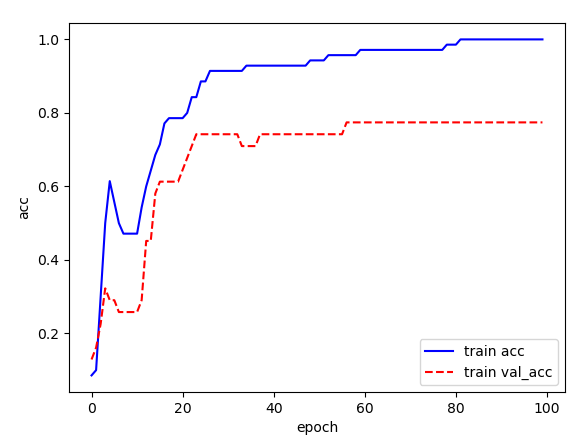
#predict
pred_data = x_data[:1] # 한개만
pred = np.argmax(model.predict(pred_data))
print(pred) # 0
print()
pred_datas = x_data[:5] # 여러개
preds = [np.argmax(i) for i in model.predict(pred_datas)]
print('예측값 : ', preds)
# 예측값 : [0, 0, 3, 0, 0]
print('실제값: ', y_data[:5].flatten())
# 실제값: [0. 0. 3. 0. 0.]
# 새로운 data
print(x_data[:1])
new_data = [[1., 0., 0., 1., 0., 0., 1., 1., 1., 1., 0., 0., 4., 0., 0., 1.]]
new_pred = np.argmax(model.predict(new_data))
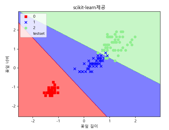
print('예측값 : ', new_pred) # 예측값 : 0다항분류 softmax + roc curve
: iris dataset으로 분류 모델 작성 후 ROC curve 출력
* ke18_iris.py
- 데이터 수집
import numpy as np
import matplotlib.pyplot as plt
from sklearn.datasets import load_iris
from sklearn.model_selection import train_test_split
from sklearn.preprocessing import OneHotEncoder, StandardScaler

iris = load_iris() # iris dataset
print(iris.DESCR)

x = iris.data # feature
print(x[:2])
# [[5.1 3.5 1.4 0.2]
#  [4.9 3.  1.4 0.2]]
y = iris.target # label
print(y)
# [0 0 0 0 0 0 0 0 0 0 0 0 0 0 0 0 0 0 0 0 0 0 0 0 0 0 0 0 0 0 0 0 0 0 0 0 0
#  0 0 0 0 0 0 0 0 0 0 0 0 0 1 1 1 1 1 1 1 1 1 1 1 1 1 1 1 1 1 1 1 1 1 1 1 1
#  1 1 1 1 1 1 1 1 1 1 1 1 1 1 1 1 1 1 1 1 1 1 1 1 1 1 2 2 2 2 2 2 2 2 2 2 2
#  2 2 2 2 2 2 2 2 2 2 2 2 2 2 2 2 2 2 2 2 2 2 2 2 2 2 2 2 2 2 2 2 2 2 2 2 2
#  2 2]
print(set(y)) # 집합
# {0, 1, 2}

names = iris.target_names
print(names)  # ['setosa' 'versicolor' 'virginica']

feature_iris = iris.feature_names
print(feature_iris) # ['sepal length (cm)', 'sepal width (cm)', 'petal length (cm)', 'petal width (cm)']
- label 원-핫 인코딩
one_hot = OneHotEncoder() # to_categorical() ..
y = one_hot.fit_transform(y[:, np.newaxis]).toarray()
print(y[:2])
# [[1. 0. 0.]
#  [1. 0. 0.]]
- feature 표준화
scaler = StandardScaler()
x_scaler = scaler.fit_transform(x)
print(x_scaler[:2])
# [[-0.90068117  1.01900435 -1.34022653 -1.3154443 ]
#  [-1.14301691 -0.13197948 -1.34022653 -1.3154443 ]]
- train / test
x_train, x_test, y_train, y_test = train_test_split(x_scaler, y, test_size=0.3, random_state=1)
n_features = x_train.shape[1] # 열
n_classes = y_train.shape[1]  # 열
print(n_features, n_classes)  # 4 3 => input, output수
- n의 개수 만큼 모델 생성 함수
from tensorflow.keras.models import Sequential
from tensorflow.keras.layers import Dense

def create_custom_model(input_dim, output_dim, out_node, n, model_name='model'):
    def create_model():
        model = Sequential(name = model_name)
        for _ in range(n): # layer 생성
            model.add(Dense(out_node, input_dim = input_dim, activation='relu'))

        model.add(Dense(output_dim, activation='softmax'))
        model.compile(optimizer='adam', loss='categorical_crossentropy', metrics=['acc'])
        return model
    return create_model # 주소 반환(클로저)
models = [create_custom_model(n_features, n_classes, 10, n, 'model_{}'.format(n)) for n in range(1, 4)]
# layer수가 2 ~ 5개 인 모델 생성
for create_model in models:
print('-------------------------')
create_model().summary()
# Total params: 83
# Total params: 193
# Total params: 303
- train
history_dict = {}

for create_model in models: # 각 모델 loss, acc 출력
    model = create_model()
    print('Model names :', model.name)
    # 훈련
    history = model.fit(x_train, y_train, batch_size=5, epochs=50, verbose=0, validation_split=0.3)
    # 평가
    score = model.evaluate(x_test, y_test)
    print('test dataset loss', score[0])
    print('test dataset acc', score[1])
    history_dict[model.name] = [history, model]

print(history_dict)
# {'model_1': [<tensorflow.python.keras.callbacks.History object at 0x00000273BA4E7280>, <tensorflow.python.keras.engine.sequential.Sequential object at 0x00000273B9B22A90>], ...}
- 시각화
fig, (ax1, ax2) = plt.subplots(2, 1, figsize=(8, 6))
print(fig, ax1, ax2)

for model_name in history_dict: # 각 모델의 acc, val_acc, val_loss
    print('h_d :', history_dict[model_name][0].history['acc'])

    val_acc = history_dict[model_name][0].history['val_acc']
    val_loss = history_dict[model_name][0].history['val_loss']
    ax1.plot(val_acc, label=model_name)
    ax2.plot(val_loss, label=model_name)
    ax1.set_ylabel('validation acc')
    ax2.set_ylabel('validation loss')
    ax2.set_xlabel('epochs')
    ax1.legend()
    ax2.legend()

plt.show()
=> model1 < model2 < model3 모델 순으로 성능 우수
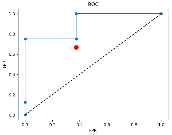
- 분류 모델에 대한 성능 평가 : ROC curve
plt.figure()
plt.plot([0, 1], [0, 1], 'k--')

from sklearn.metrics import roc_curve, auc

for model_name in history_dict: # 각 모델의 모델
    model = history_dict[model_name][1]
    y_pred = model.predict(x_test)
    fpr, tpr, _ = roc_curve(y_test.ravel(), y_pred.ravel())
    plt.plot(fpr, tpr, label='{}, AUC value : {:.3}'.format(model_name, auc(fpr, tpr)))

plt.xlabel('fpr')
plt.ylabel('tpr')
plt.title('ROC curve')
plt.legend()
plt.show()
- k-fold 교차 검증 - over fitting 방지
from tensorflow.keras.wrappers.scikit_learn import KerasClassifier
from sklearn.model_selection import cross_val_score

creater_model = create_custom_model(n_features, n_classes, 10, 3)
estimator = KerasClassifier(build_fn = create_model, epochs=50, batch_size=10, verbose=2)
scores = cross_val_score(estimator, x_scaler, y, cv=10)
print('accuracy : {:0.2f}(+/-{:0.2f})'.format(scores.mean(), scores.std()))
# accuracy : 0.92(+/-0.11)
- 모델 3의 성능이 가장 우수
model = Sequential()

model.add(Dense(10, input_dim=4, activation='relu'))
model.add(Dense(10, activation='relu'))
model.add(Dense(10, activation='relu'))
model.add(Dense(3, activation='softmax'))

model.compile(loss='categorical_crossentropy', optimizer='adam',  metrics=['acc'])
model.fit(x_train, y_train, epochs=50, batch_size=10, verbose=2)
print(model.evaluate(x_test, y_test))
# [0.20484387874603271, 0.8888888955116272]

y_pred = np.argmax(model.predict(x_test), axis=1)
print('예측값 :', y_pred)
# 예측값 : [0 1 1 0 2 2 2 0 0 2 1 0 2 1 1 0 1 2 0 0 1 2 2 0 2 1 0 0 1 2 1 2 1 2 2 0 1
#  0 1 2 2 0 1 2 1]

real_y = np.argmax(y_test, axis=1).reshape(-1, 1)
print('실제값 :', real_y.ravel())
# 실제값 : [0 1 1 0 2 1 2 0 0 2 1 0 2 1 1 0 1 1 0 0 1 1 1 0 2 1 0 0 1 2 1 2 1 2 2 0 1
#  0 1 2 2 0 2 2 1]

print('분류 실패 수 :', (y_pred != real_y.ravel()).sum())
# 분류 실패 수 : 5
from sklearn.metrics import confusion_matrix, classification_report, accuracy_score
print(confusion_matrix(real_y, y_pred))
# [[14  0  0]
#  [ 0 17  1]
#  [ 0  1 12]]

print(accuracy_score(real_y, y_pred)) # 0.9555555555555556
print(classification_report(real_y, y_pred))
#               precision    recall  f1-score   support
#
#            0       1.00      1.00      1.00        14
#            1       0.94      0.94      0.94        18
#            2       0.92      0.92      0.92        13
#
#     accuracy                           0.96        45
#    macro avg       0.96      0.96      0.96        45
# weighted avg       0.96      0.96      0.96        45
- 새로운 값으로 예측
new_x = [[5.5, 3.3, 1.2, 1.3], [3.5, 3.3, 0.2, 0.3], [1.5, 1.3, 6.2, 6.3]]
new_x = StandardScaler().fit_transform(new_x)
new_pred = model.predict(new_x)
print('예측값 :', np.argmax(new_pred, axis=1).reshape(-1, 1).flatten()) # 예측값 : [1 0 2]
숫자 이미지(MNIST) dataset으로 image 분류 모델
: 숫자 이미지를 metrics로 만들어 이미지에 대한 분류 결과를 mapping한 dataset
- mnist dataset
sdc-james.gitbook.io/onebook/4.-and/5.1./5.1.3.-mnist-dataset
5.1.3. MNIST Dataset 소개
sdc-james.gitbook.io
* ke19_mist.py
import tensorflow as tf
import sys

(x_train, y_train),(x_test, y_test) = tf.keras.datasets.mnist.load_data()
print(len(x_train), len(x_test),len(y_train), len(y_test)) # 60000 10000 60000 10000
print(x_train.shape, y_train.shape)                        # (60000, 28, 28) (60000,)
print(x_train[0])

for i in x_train[0]:
    for j in i:
        sys.stdout.write('%s   '%j)
    sys.stdout.write('\n')

x_train = x_train.reshape(60000, 784).astype('float32') # 3차원 -> 2차원
x_test = x_test.reshape(10000, 784).astype('float32')
import matplotlib.pyplot as plt
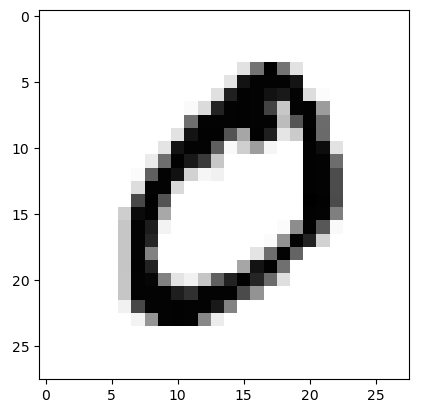
plt.imshow(x_train[0].reshape(28,28), cmap='Greys')
plt.show()
print(y_train[0]) # 5
plt.imshow(x_train[1].reshape(28,28), cmap='Greys')
plt.show()
print(y_train[1]) # 0
# 정규화
x_train /= 255 # 0 ~ 255 사이의 값을 0 ~ 1사이로 정규화
x_test /= 255
print(x_train[0])
print(set(y_train)) # {0, 1, 2, 3, 4, 5, 6, 7, 8, 9}
y_train = tf.keras.utils.to_categorical(y_train, 10) # one-hot encoding
y_test = tf.keras.utils.to_categorical(y_test, 10) # one-hot encoding
print(y_train[0]) # [0. 0. 0. 0. 0. 1. 0. 0. 0. 0.]
- train dataset의 일부를 validation dataset
x_val = x_train[50000:60000]
y_val = y_train[50000:60000]
x_train = x_train[0:50000]
y_train = y_train[0:50000]
print(x_val.shape, ' ', x_train.shape) # (10000, 28, 28)   (50000, 28, 28)
print(y_val.shape, ' ', y_train.shape) # (10000, 10)   (50000, 10)

model = tf.keras.Sequential()

model.add(tf.keras.layers.Dense(512, input_shape=(784, )))
model.add(tf.keras.layers.Activation('relu'))
model.add(tf.keras.layers.Dropout(0.2)) # 20% drop -> over fitting 방지

model.add(tf.keras.layers.Dense(512))
# model.add(tf.keras.layers.Dense(512, kernel_regularizer=tf.keras.regularizers.l2(0.001))) # 가중치 규제
model.add(tf.keras.layers.Activation('relu'))
model.add(tf.keras.layers.Dropout(0.2))

model.add(tf.keras.layers.Dense(10))
model.add(tf.keras.layers.Activation('softmax'))

model.compile(optimizer=tf.keras.optimizers.Adam(lr=0.01), loss='categorical_crossentropy', metrics=['accuracy'])
print(model.summary()) # Total params: 669,706
- 훈련
from tensorflow.keras.callbacks import EarlyStopping
e_stop = EarlyStopping(patience=5, monitor='loss')

history = model.fit(x_train, y_train, epochs=1000, batch_size=256, validation_data=(x_val, y_val),\
                    callbacks=[e_stop], verbose=1)
print(history.history.keys()) # dict_keys(['loss', 'accuracy', 'val_loss', 'val_accuracy'])


print('loss :', history.history['loss'],', val_loss :', history.history['val_loss'])
print('accuracy :', history.history['accuracy'],', val_accuracy :', history.history['val_accuracy'])

plt.plot(history.history['loss'], label='loss')
plt.plot(history.history['val_loss'], label='val_loss')
plt.xlabel('epochs')
plt.ylabel('loss')
plt.legend()
plt.show()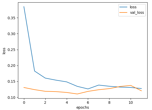
plt.plot(history.history['accuracy'], label='accuracy')
plt.plot(history.history['val_accuracy'], label='val_accuracy')
plt.xlabel('epochs')
plt.ylabel('accuracy')
plt.legend()
plt.show()
score = model.evaluate(x_test, y_test)
print('score loss :', score[0])
# score loss : 0.12402850389480591

print('score accuracy :', score[1])
# score accuracy : 0.9718999862670898

model.save('ke19.hdf5')

model = tf.keras.models.load_model('ke19.hdf5')
- 예측
pred = model.predict(x_test[:1])
print('예측값 :', pred)
# 예측값 : [[4.3060442e-27 3.1736336e-14 3.9369942e-17 3.7753089e-14 6.8288101e-22
#   5.2651956e-21 2.7473105e-33 1.0000000e+00 1.6139679e-21 1.6997739e-14]]
# [7]

import numpy as np
print(np.argmax(pred, 1))
print('실제값 :', y_test[:1])
# 실제값 : [[0. 0. 0. 0. 0. 0. 0. 1. 0. 0.]]
print('실제값 :', np.argmax(y_test[:1], 1))
# 실제값 : [7]
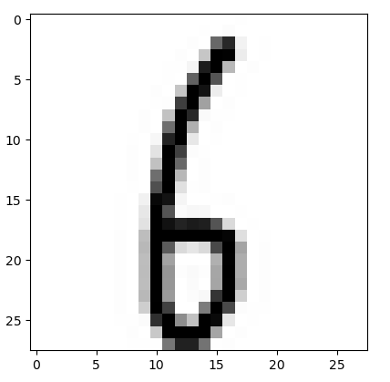
- 새로운 이미지로 분류
from PIL import Image
im = Image.open('num.png')
img = np.array(im.resize((28, 28), Image.ANTIALIAS).convert('L'))
print(img, img.shape) # (28, 28)

plt.imshow(img, cmap='Greys')
plt.show()
from PIL import Image
Image.open('파일경로') : 이미지 파일 open.
Image.ANTIALIAS : 높은 해상도의 사진 또는 영상을 낮은 해상도로 변환하거나 나타낼 시의 깨짐을 최소화 시켜주는 방법.
convert('L') : grey scale로 변환.
data = img.reshape([1, 784])
data = data/255  # 정규화
print(data)

new_pred = model.predict(data)
print('new_pred :', new_pred)
# new_pred : [[4.92454797e-04 1.15842435e-04 6.54530758e-03 5.23587340e-04
#   3.31552816e-04 5.98833859e-01 3.87458414e-01 9.34154059e-07
#   5.55288605e-03 1.45193975e-04]]
print('new_pred :', np.argmax(new_pred, 1))
# new_pred : [5]
이미지 분류 패션 MNIST
- Fashion MNIST
www.kaggle.com/zalando-research/fashionmnist
Fashion MNIST
An MNIST-like dataset of 70,000 28x28 labeled fashion images
www.kaggle.com
* ke20_fasion.py
import tensorflow as tf
from tensorflow import keras
import numpy as np
import matplotlib.pyplot as plt

fashion_mnist = tf.keras.datasets.fashion_mnist
(train_image, train_labels), (test_image, test_labels) = fashion_mnist.load_data()
print(train_image.shape, train_labels.shape, test_image.shape)
# (60000, 28, 28) (60000,)

print(set(train_labels))
# {0, 1, 2, 3, 4, 5, 6, 7, 8, 9}
class_names = ['T-shirt/top', 'Trouser', 'Pullover', 'Dress', 'Coat', 'Sandal', 'Shirt', 'Sneaker', 'Bag', 'Ankle boot']

plt.imshow(train_image[0])
plt.colorbar()
plt.show()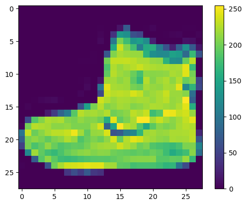
plt.figure(figsize=(10, 10))
for i in range(25):
    plt.subplot(5, 5, i+1)
    plt.xticks([])
    plt.yticks([])
    plt.xlabel(class_names[train_labels[i]])
    plt.imshow(train_image[i])

plt.show()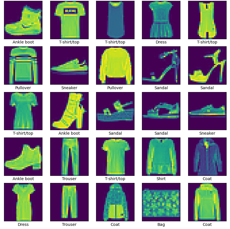
- 정규화
# print(train_image[0])
train_image = train_image/255
# print(train_image[0])
test_image = test_image/255
- 모델 구성
model = tf.keras.Sequential([
    tf.keras.layers.Flatten(input_shape = (28, 28)), # 차원 축소. 일반적으로 생략 가능(자동 동작).
    tf.keras.layers.Dense(512, activation = tf.nn.relu),
    tf.keras.layers.Dense(128, activation = tf.nn.relu),
    tf.keras.layers.Dense(10, activation = tf.nn.softmax)
    ])

model.compile(optimizer='adam', loss='sparse_categorical_crossentropy', metrics=['accuracy']) # label에 대해서 one-hot encoding

model.fit(train_image, train_labels, batch_size=128, epochs=5, verbose=1)

model.save('ke20.hdf5')

model = tf.keras.models.load_model('ke20.hdf5')
model.compile(optimizer=, loss='sparse_categorical_crossentropy', metrics=) : label에 대해서 one-hot encoding
test_loss, test_acc = model.evaluate(test_image, test_labels)
print('loss :', test_loss)
# loss : 0.34757569432258606
print('acc :', test_acc)
# acc : 0.8747000098228455

pred = model.predict(test_image)
print(pred[0])
# [8.5175507e-06 1.2854183e-06 8.2240956e-07 1.3558407e-05 2.0901878e-06
#  1.3651027e-02 7.2083326e-06 4.6001904e-02 2.0302361e-05 9.4029325e-01]
print('예측값 :', np.argmax(pred[0]))
# 예측값 : 9
print('실제값 :', test_labels[0])
# 실제값 : 9
- 각 이미지 출력용 함수
def plot_image(i, pred_arr, true_label, img):
    pred_arr, true_label, img = pred_arr[i], true_label[i], img[i]
    plt.xticks([])
    plt.yticks([])
    plt.imshow(img, cmap='Greys')

    pred_label = np.argmax(pred_arr)
    if pred_label == true_label:
        color = 'blue'
    else:
        color = 'red'

    plt.xlabel('{} {:2.0f}% ({})'.format(class_names[pred_label], 100 * np.max(pred_arr), \
                                         class_names[true_label]), color = color)

i = 0
plt.figure(figsize = (6, 3))
plt.subplot(1, 2, 1)
plot_image(i, pred, test_labels, test_image)
plt.show()
def plot_value_arr(i, pred_arr, true_label):
    pred_arr, true_label = pred_arr[i], true_label[i]
    thisplot = plt.bar(range(10), pred_arr)
    plt.ylim([0, 1])
    pred_label = np.argmax(pred_arr)
    thisplot[pred_label].set_color('red')
    thisplot[true_label].set_color('blue')


i = 12
plt.figure(figsize = (6, 3))
plt.subplot(1, 2, 1)
plot_image(i, pred, test_labels, test_image)
plt.subplot(1, 2, 2)
plot_value_arr(i, pred, test_labels)
plt.show()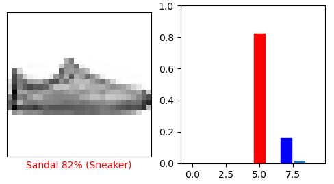
합성곱 신경망 (Convolutional Neural Network, CNN)
: 원본 이미지(행렬)를 CNN의 필터(행렬)로 합성 곱을 하여 행렬 크기를 줄여 분류한다.
: 부하를 줄이며, 이미지 분류 향상에 영향을 준다.
- CNN
[머신 러닝/딥 러닝] 합성곱 신경망 (Convolutional Neural Network, CNN)과 학습 알고리즘
1. 이미지 처리와 필터링 기법 필터링은 이미지 처리 분야에서 광범위하게 이용되고 있는 기법으로써, 이미지에서 테두리 부분을 추출하거나 이미지를 흐릿하게 만드는 등의 기능을 수행하기
untitledtblog.tistory.com
=> input -> [ conv -> relu -> pooling ] -> ... -> Flatten -> Dense -> ... -> output
- MNIST dataset으로 cnn진행
* ke21_cnn.py
import tensorflow as tf
from tensorflow.keras import datasets, models, layers

(train_images, train_labels),(test_images, test_labels) = datasets.mnist.load_data()
print(train_images.shape)                    # (60000, 28, 28)
from tensorflow.keras import datasets
datasets.mnist.load_data() : mnist dataset
- CNN : 3차원을 4차원(+channel(RGB))으로 구조 변경
train_images = train_images.reshape((60000, 28, 28, 1))
print(train_images.shape, train_images.ndim) # (60000, 28, 28, 1) 4
train_images = train_images / 255.0 # 정규화
print(train_images[0])

test_images = test_images.reshape((10000, 28, 28, 1))
test_images = test_images / 255.0 # 정규화

print(train_labels[:3]) # [5 0 4]
channel 수 : 흑백 - 1, 컬러 - 3
- 모델
input_shape = (28, 28, 1)
model = models.Sequential()

# 형식 : tf.keras.layers.Conv2D(filters, kernel_size, strides=(1, 1), padding='valid', ...
model.add(layers.Conv2D(64, kernel_size = (3, 3), strides=(1, 1), padding ='valid',\
                        activation='relu', input_shape=input_shape))
model.add(layers.MaxPooling2D(pool_size=(2, 2), strides=None))
model.add(layers.Dropout(0.2))

model.add(layers.Conv2D(32, kernel_size = (3, 3), strides=(1, 1), padding ='valid', activation='relu'))
model.add(layers.MaxPooling2D(pool_size=(2, 2), strides=None))
model.add(layers.Dropout(0.2))

model.add(layers.Conv2D(16, kernel_size = (3, 3), strides=(1, 1), padding ='valid', activation='relu'))
model.add(layers.MaxPooling2D(pool_size=(2, 2), strides=None))
model.add(layers.Dropout(0.2))

model.add(layers.Flatten()) # Fully Connect layer - CNN 처리된 데이터를 1차원 자료로 변경
from tensorflow.keras import layers
layers.Conv2D(output수, kernel_size=, strides=, padding=, activation=, input_shape=) : CNN Conv
strides : 보폭, None - pool_size와 동일
padding : valid - 영역 밖에 0으로 채우지 않고 곱 진행, same - 영역 밖에 0으로 채우고 곱 진행.
layers.MaxPooling2D(pool_size=, strides=) : CNN Pooling
layers.Flatten() : Fully Connect layer - CNN 처리된 데이터를 1차원 자료로 변경
- Conv2D
www.tensorflow.org/api_docs/python/tf/keras/layers/Conv2D
tf.keras.layers.Conv2D | TensorFlow Core v2.4.1
2D convolution layer (e.g. spatial convolution over images).
www.tensorflow.org
- 모델
model.add(layers.Dense(64, activation='relu'))
model.add(layers.Dense(32, activation='relu'))
model.add(layers.Dense(10, activation='softmax'))

print(model.summary())
- 학습설정
model.compile(optimizer='adam', loss='sparse_categorical_crossentropy', metrics=['accuracy'])
# label에 대해서 one-hot encoding
model.compile(optimizer='', loss='sparse_categorical_crossentropy', metrics=) : label에 대해서 one-hot encoding.
- 훈련
from tensorflow.keras.callbacks import EarlyStopping
early_stop = EarlyStopping(monitor='val_loss', patience=3) # 조기 종료

histoy = model.fit(train_images, train_labels, batch_size=128, epochs=100, verbose=1, validation_split=0.2,\
                   callbacks = [early_stop])
- 평가
train_loss, train_acc = model.evaluate(train_images, train_labels)
print('train_loss :', train_loss)
print('train_acc :', train_acc)

test_loss, test_acc = model.evaluate(test_images, test_labels)
print('test_loss :', test_loss)
print('test_acc :', test_acc)
# test_loss : 0.06314415484666824
# test_acc : 0.9812999963760376
- 모델 저장
model.save('ke21.h5')

model = tf.keras.models.load_model('ke21.h5')

import pickle
histoy = histoy.history # loss, acc

with open('data.pickle', 'wb') as f: # 파일 저장
    pickle.dump(histoy)              # 객체 저장

with open('data.pickle', 'rb') as f: # 파일 읽기
    history = pickle.load(f)         # 객체 읽기
import pickle
pickle.dump(객체) : 객체 저장
pickle.load(f) : 객체 불러오기
- 예측
import numpy as np
print('예측값 :', np.argmax(model.predict(test_images[:1])))
print('예측값 :', np.argmax(model.predict(test_images[[0]])))
print('실제값 :', test_labels[0])
# 예측값 : 7
# 예측값 : 7
# 실제값 : 7

print('예측값 :', np.argmax(model.predict(test_images[[1]])))
print('실제값 :', test_labels[1])
# 예측값 : 2
# 실제값 : 2
- acc와 loss로 시각화
import matplotlib.pyplot as plt
def plot_acc(title = None):
plt.plot(history['accuracy'])
plt.plot(history['val_accuracy'])
if title is not None:
plt.title(title)
plt.ylabel(title)
plt.xlabel('epoch')
plt.legend(['train data', 'validation data'], loc = 0)
plot_acc('accuracy')
plt.show()
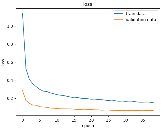
def plot_loss(title = None):
plt.plot(history['loss'])
plt.plot(history['val_loss'])
if title is not None:
plt.title(title)
plt.ylabel(title)
plt.xlabel('epoch')
plt.legend(['train data', 'validation data'], loc = 0)
plot_loss('loss')
plt.show()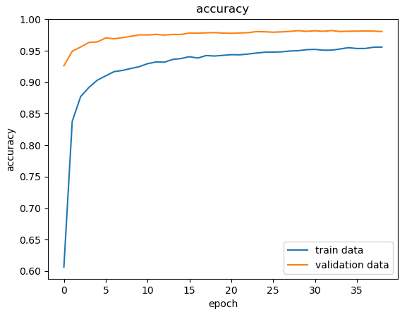
Tensor : image process, CNN
Daum 카페
cafe.daum.net
- 딥러닝 적용사례
딥러닝의 30가지 적용 사례
비전문가들도 이해할 수 있을 구체적 예시 | *본 글은 Yaron Hadad의 블로그 'http://www.yaronhadad.com/deep-learning-most-amazing-applications/'를 동의 하에 번역하였습니다. 최근 몇 년간 딥러닝은 컴퓨터 비전부
brunch.co.kr
CNN - 이미지 분류
RNN - 시계열. ex) 자연어, ..
GAN - 창조
- CNN
CNN, Convolutional Neural Network 요약
Convolutional Neural Network, CNN을 정리합니다.
taewan.kim
* tf_cnn_mnist_subclassing.ipynb
- MNIST로 cnn 연습
import tensorflow as tf
from tensorflow.keras import datasets, models, layers, Model
from tensorflow.keras.layers import Dense, Flatten, Conv2D, MaxPool2D, Dropout

(train_images, train_labels),(test_images, test_labels) = tf.keras.datasets.mnist.load_data()
print(train_images.shape)                    # (60000, 28, 28)

train_images = train_images.reshape((60000, 28, 28, 1))
print(train_images.shape, train_images.ndim) # (60000, 28, 28, 1) 4
train_images = train_images / 255.0 # 정규화
#print(train_images[0])

test_images = test_images.reshape((10000, 28, 28, 1))
test_images = test_images / 255.0 # 정규화

print(train_labels[:3]) # [5 0 4]
- 데이터 섞기
import numpy as np
x = np.random.sample((5,2))
print(x)
'''
[[0.19516051 0.38639727]
 [0.89418845 0.05847686]
 [0.16835491 0.11172334]
 [0.8109798  0.68812899]
 [0.03361333 0.83081767]]
'''
dset = tf.data.Dataset.from_tensor_slices(x)
print(dset) # <TensorSliceDataset shapes: (2,), types: tf.float64>
dset = tf.data.Dataset.from_tensor_slices(x).shuffle(1000).batch(2) # batch(묶음수), shuffle(buffer수) : 섞음
print(dset) # <BatchDataset shapes: (None, 2), types: tf.float64>
for a in dset:
    print(a)
    '''
    tf.Tensor(
[[0.93919653 0.52250196]
 [0.44236167 0.53000042]
 [0.69057762 0.32003977]], shape=(3, 2), dtype=float64)
tf.Tensor(
[[0.09166211 0.67060753]
 [0.39949866 0.57685399]], shape=(2, 2), dtype=float64)
'''tf.data.Dataset.from_tensor_slices(x).shuffle(1000).batch(3) : batch(묶음수), shuffle(buffer수) : 섞음
- MNIST이 train data를 섞기
train_ds = tf.data.Dataset.from_tensor_slices(((train_images, train_labels))).shuffle(60000).batch(28)
test_ds = tf.data.Dataset.from_tensor_slices(((test_images, test_labels))).batch(28)
print(train_ds)
print(test_ds)
- 모델 생성방법 : subclassing API 사용
class MyModel(Model):
    def __init__(self):
        super(MyModel, self).__init__()
        self.conv1 = Conv2D(filters=32, kernel_size = [3,3], padding ='valid', activation='relu')
        self.pool1 = MaxPool2D((2, 2))

        self.conv2 = Conv2D(filters=32, kernel_size = [3,3], padding ='valid', activation='relu')
        self.pool2 = MaxPool2D((2, 2))

        self.flatten = Flatten(dtype='float32')

        self.d1 = Dense(64, activation='relu')
        self.drop1 = Dropout(rate = 0.3)
        self.d2 = Dense(10, activation='softmax')

    def call(self, inputs):
        net = self.conv1(inputs)
        net = self.pool1(net)
        net = self.conv2(net)
        net = self.pool2(net)
        net = self.flatten(net)
        net = self.d1(net)
        net = self.drop1(net)
        net = self.d2(net)
        return net

model = MyModel()
temp_inputs = tf.keras.Input(shape=(28, 28, 1))
model(temp_inputs)
print(model.summary())
'''
Layer (type)                 Output Shape              Param #
=================================================================
conv2d_2 (Conv2D)            multiple                  320
_________________________________________________________________
max_pooling2d (MaxPooling2D) multiple                  0
_________________________________________________________________
conv2d_3 (Conv2D)            multiple                  9248
_________________________________________________________________
max_pooling2d_1 (MaxPooling2 multiple                  0
_________________________________________________________________
flatten (Flatten)            multiple                  0
_________________________________________________________________
dense (Dense)                multiple                  51264
_________________________________________________________________
dropout (Dropout)            multiple                  0
_________________________________________________________________
dense_1 (Dense)              multiple                  650
=================================================================
Total params: 61,482
'''
- 일반적 모델학습 방법1
loss_object = tf.keras.losses.SparseCategoricalCrossentropy()
optimizer = tf.keras.optimizers.Adam()

# 일반적 모델학습 방법1
model.compile(optimizer=optimizer, loss=loss_object, metrics=['acc'])
model.fit(train_images, train_labels, batch_size=128, epochs=5, verbose=2, max_queue_size=10, workers=1, use_multiprocessing=True)
# use_multiprocessing : 프로세스 기반의
score = model.evaluate(test_images, test_labels)
print('test loss :', score[0])
print('test acc :', score[1])
# test loss : 0.028807897120714188
# test acc : 0.9907000064849854

import numpy as np
print('예측값 :', np.argmax(model.predict(test_images[:2]), 1))
print('실제값 :', test_labels[:2])
# 예측값 : [7 2]
# 실제값 : [7 2]
- 모델 학습방법2: GradientTape
train_loss = tf.keras.metrics.Mean()
train_accuracy = tf.keras.metrics.SparseCategoricalAccuracy()

test_loss = tf.keras.metrics.Mean()
test_accuracy = tf.keras.metrics.SparseCategoricalAccuracy()

@tf.function
def train_step(images, labels):
    with tf.GradientTape() as tape:
        predictions = model(images)
        loss = loss_object(labels, predictions)

    gradients = tape.gradient(loss, model.trainable_variables)
    optimizer.apply_gradients(zip(gradients, model.trainable_variables))
    train_loss(loss) # 가중치 평균 계산       loss = loss_object(labels, predictions)
    train_accuracy(labels, predictions)

@tf.function
def test_step(images, labels):
    predictions = model(images)
    t_loss = loss_object(labels, predictions)
    test_loss(t_loss)
    test_accuracy(labels, predictions)

EPOCHS = 5

for epoch in range(EPOCHS):
    for train_images, train_labels in train_ds:
        train_step(train_images, train_labels)

    for test_images, test_labels in test_ds:
        test_step(test_images, test_labels)

    templates = 'epochs:{}, train_loss:{}, train_acc:{}, test_loss:{}, test_acc:{}'
    print(templates.format(epoch + 1, train_loss.result(), train_accuracy.result()*100,\
                           test_loss.result(), test_accuracy.result()*100))

print('예측값 :', np.argmax(model.predict(test_images[:2]), 1))
print('실제값 :', test_labels[:2].numpy())
# 예측값 : [3 4]
# 실제값 : [3 4]
- image data generator
: 샘플수가 적을 경우 사용.
[Keras] CNN ImageDataGenerator : 손글씨 글자 분류
안녕하세요. 이전 포스팅을 통해서 CNN을 활용한 직접 만든 손글씨 이미지 분류 작업을 진행했습니다. 생각보다 데이터가 부족했음에도 80% 정도의 정확도를 보여주었습니다. 이번 포스팅에서는
chancoding.tistory.com
+ 이미지 보강
* tf_cnn_image_generator.ipynb
import tensorflow as tf
from tensorflow.keras.datasets import mnist
from tensorflow.keras.utils import to_categorical
from tensorflow.keras.callbacks import ModelCheckpoint, EarlyStopping
import matplotlib.pyplot as plt
import numpy as np
import sys
np.random.seed(0)
tf.random.set_seed(3)
(x_train, y_train), (x_test, y_test) = mnist.load_data()
x_train = x_train.reshape(-1, 28, 28, 1).astype('float32') /255
x_test = x_test.reshape(-1, 28, 28, 1).astype('float32') /255
#print(x_train[0])
# print(y_train[0])
y_train = to_categorical(y_train)
print(y_train[0]) # [0. 0. 0. 0. 0. 1. 0. 0. 0. 0.]
y_test = to_categorical(y_test)
- 이미지 보강 클래스 : 기존 이미지를 좌우대칭, 회전, 기울기, 이동 등을 통해 이미지의 양을 늘림
from tensorflow.keras.preprocessing.image import ImageDataGenerator
# 연습
img_gen = ImageDataGenerator(
    rotation_range = 10, # 회전 범위
    zoom_range = 0.1, # 확대 축소
    shear_range = 0.5, # 축 기준
    width_shift_range = 0.1, # 평행이동
    height_shift_range = 0.1, # 수직이동
    horizontal_flip = True, # 좌우 반전
    vertical_flip = False # 상하 반전
)
augument_size = 100
x_augument = img_gen.flow(np.tile(x_train[0].reshape(28*28), 100).reshape(-1, 28, 28, 1),
                          np.zeros(augument_size),
                          batch_size = augument_size,
                          shuffle = False).next()[0]
plt.figure(figsize=(10, 10))
for c in range(100):
    plt.subplot(10, 10, c+1)
    plt.axis('off')
    plt.imshow(x_augument[c].reshape(28, 28), cmap='gray')
plt.show()
img_generate = ImageDataGenerator(
    rotation_range = 10, # 회전 범위
    zoom_range = 0.1, # 확대 축소
    shear_range = 0.5, # 축 기준
    width_shift_range = 0.1, # 평행이동
    height_shift_range = 0.1, # 수직이동
    horizontal_flip = False, # 좌우 반전
    vertical_flip = False # 상하 반전
)
augument_size = 30000 # 변형 이미지 3만개
randIdx = np.random.randint(x_train.shape[0], size = augument_size)
x_augment = x_train[randIdx].copy()
y_augment = y_train[randIdx].copy()

x_augument = img_generate.flow(x_augment,
                          np.zeros(augument_size),
                          batch_size = augument_size,
                          shuffle = False).next()[0]

# 원래 이미지에 증식된 이미지를 추가
x_train = np.concatenate((x_train, x_augment))
y_train = np.concatenate((y_train, y_augment))
print(x_train.shape) # (90000, 28, 28, 1)
model = tf.keras.models.Sequential([
    tf.keras.layers.Conv2D(filters=32, kernel_size=(3, 3), input_shape=(28, 28, 1), padding='same', activation='relu'),
    tf.keras.layers.MaxPooling2D(pool_size=(2,2)),
    tf.keras.layers.Dropout(0.3),

    tf.keras.layers.Conv2D(filters=32, kernel_size=(3, 3), input_shape=(28, 28, 1), padding='same', activation='relu'),
    tf.keras.layers.MaxPooling2D(pool_size=(2,2)),

    tf.keras.layers.Flatten(),

    tf.keras.layers.Dense(units=128, activation='relu'),
    tf.keras.layers.Dropout(0.3),
    tf.keras.layers.Dense(units=64, activation='relu'),
    tf.keras.layers.Dropout(0.3),
    tf.keras.layers.Dense(units=10, activation='softmax')
])
model.compile(optimizer='Adam', loss='categorical_crossentropy', metrics=['accuracy'])
print(model.summary())
'''
Layer (type)                 Output Shape              Param #
=================================================================
conv2d_8 (Conv2D)            (None, 28, 28, 32)        320
_________________________________________________________________
max_pooling2d_7 (MaxPooling2 (None, 14, 14, 32)        0
_________________________________________________________________
dropout_6 (Dropout)          (None, 14, 14, 32)        0
_________________________________________________________________
conv2d_9 (Conv2D)            (None, 14, 14, 32)        9248
_________________________________________________________________
max_pooling2d_8 (MaxPooling2 (None, 7, 7, 32)          0
_________________________________________________________________
flatten_1 (Flatten)          (None, 1568)              0
_________________________________________________________________
dense_2 (Dense)              (None, 128)               200832
_________________________________________________________________
dropout_7 (Dropout)          (None, 128)               0
_________________________________________________________________
dense_3 (Dense)              (None, 64)                8256
_________________________________________________________________
dropout_8 (Dropout)          (None, 64)                0
_________________________________________________________________
dense_4 (Dense)              (None, 10)                650
=================================================================
Total params: 219,306
'''
early_stop = EarlyStopping(monitor='val_loss', patience=3)
history = model.fit(x_train, y_train, validation_split=0.2, epochs=100, batch_size=64, \
verbose=2, callbacks=[early_stop])
print('Accuracy : %.3f'%(model.evaluate(x_test, y_test)[1]))
# Accuracy : 0.992print('accuracy :%.3f'%(model.evaluate(x_test, y_test)[1]))
# accuracy :0.992
# 시각화
plt.figure(figsize=(12,4))
plt.subplot(1, 2, 1)
plt.plot(history.history['accuracy'], marker = 'o', c='red', label='acc')
plt.plot(history.history['val_accuracy'], marker = 's', c='blue', label='val_acc')
plt.xlabel('epochs')
plt.ylim(0.5, 1)
plt.legend(loc='lower right')
plt.subplot(1, 2, 2)
plt.plot(history.history['loss'], marker = 'o', c='red', label='loss')
plt.plot(history.history['val_loss'], marker = 's', c='blue', label='val_loss')
plt.xlabel('epochs')
plt.legend(loc='upper right')
plt.show()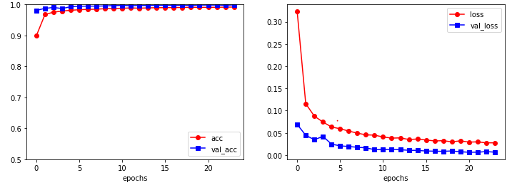
'BACK END > Deep Learning' 카테고리의 다른 글
| [딥러닝] RNN, NLP (0) | 2021.04.05 |
|---|---|
| [딥러닝] Tensorflow - 이미지 분류 (0) | 2021.04.01 |
| [딥러닝] Keras - Linear (0) | 2021.03.23 |
| [딥러닝] TensorFlow (0) | 2021.03.22 |
| [딥러닝] TensorFlow 환경설정 (0) | 2021.03.22 |