클러스터링(Clustering)
: 비지도 학습의 일종
: 계층적 군집분석
- 계층적 군집분석 종류
- 응집형 : 자료 하나하나를 군집으로 간주하고, 가까운 군집끼리 연결하는 방법. 군집의 크기를 점점 늘려가는 알고리즘. 상향식
- 분리형 : 전체 자료를 큰 군집으로 간주하고, 유의미한 부분을 분리해 나가는 방법. 군집의 크기를 점점 줄여가는 알고리즘. 하향식
k-means : 군집 수(k) 지정. 거리(유클리디안 거리 계산 법)들의 평균으로 비계층적 군집분석 진행.
- 이론
군집 분석 (Clustering analysis)
군집 분석은 각 개체의 유사성을 측정하여 높은 대상 집단을 분류하고, 군집에 속한 개체들의 유사성과 서...
blog.naver.com
* cluster1.py
import pandas as pd
import numpy as np
import matplotlib.pyplot as plt
plt.rc('font', family='malgun gothic')

np.random.seed(123)
var = ['x', 'y']
labels = ['점0','점1', '점2', '점3', '점4']
x = np.random.random_sample([5, 2]) * 10
df = pd.DataFrame(x, columns = var, index = labels)
print(df)
'''           x         y
점0  6.964692  2.861393
점1  2.268515  5.513148
점2  7.194690  4.231065
점3  9.807642  6.848297
점4  4.809319  3.921175
'''

plt.scatter(x[:, 0], x[:, 1], c='blue', marker='o')
plt.grid(True)
plt.show()
from scipy.spatial.distance import pdist, squareform

dist_vec = pdist(df, metric='euclidean') # 데이터간 거리를 유클리디안 거리계산을 사용하여 측정
print('distmatrix :', dist_vec)
# [5.3931329  1.38884785 4.89671004 2.40182631 5.09027885 7.6564396 2.99834352 3.69830057 2.40541571 5.79234641]

print(squareform(dist_vec)) # 데이터를 테이블 형태로 변경
'''
[[0.         5.3931329  1.38884785 4.89671004 2.40182631]
 [5.3931329  0.         5.09027885 7.6564396  2.99834352]
 [1.38884785 5.09027885 0.         3.69830057 2.40541571]
 [4.89671004 7.6564396  3.69830057 0.         5.79234641]
 [2.40182631 2.99834352 2.40541571 5.79234641 0.        ]]
'''

row_dist = pd.DataFrame(squareform(dist_vec))
print(row_dist)
'''
          0         1         2         3         4
0  0.000000  5.393133  1.388848  4.896710  2.401826
1  5.393133  0.000000  5.090279  7.656440  2.998344
2  1.388848  5.090279  0.000000  3.698301  2.405416
3  4.896710  7.656440  3.698301  0.000000  5.792346
4  2.401826  2.998344  2.405416  5.792346  0.000000
'''
from scipy.spatial.distance import pdist
distance=pdist(df, metric='euclidean') : 데이터간 거리를 유클리디안 거리계산을 사용하여 측정
from scipy.spatial.distance import squareform
squareform(distance) : 데이터를 테이블 형태로 변경
from scipy.cluster.hierarchy import linkage # 응집형 계층적 군집분석

row_clusters = linkage(dist_vec, method='ward') # method : complete, single, average, ..
print(row_clusters)
'''
[[0.         2.         1.38884785 2.        ]
 [4.         5.         2.65710936 3.        ]
 [1.         6.         5.45400408 4.        ]
 [3.         7.         6.64710151 5.        ]]
'''

df = pd.DataFrame(row_clusters, columns=['클러스터1', '클러스터2', '거리', '멤버 수'])
print(df)
'''
   클러스터1  클러스터2        거리  멤버 수
0    0.0    2.0  1.388848   2.0
1    4.0    5.0  2.657109   3.0
2    1.0    6.0  5.454004   4.0
3    3.0    7.0  6.647102   5.0
'''
from scipy.cluster.hierarchy import linkage
linkage(distance, method='ward') :응집형 계층적 군집분석
method : complete, single, average, ...
- linkage API
docs.scipy.org/doc/scipy/reference/generated/scipy.cluster.hierarchy.linkage.html
scipy.cluster.hierarchy.linkage — SciPy v1.6.1 Reference Guide
For method ‘single’, an optimized algorithm based on minimum spanning tree is implemented. It has time complexity \(O(n^2)\). For methods ‘complete’, ‘average’, ‘weighted’ and ‘ward’, an algorithm called nearest-neighbors chain is imple
docs.scipy.org
from scipy.cluster.hierarchy import dendrogram

dendrogram(row_clusters, labels=labels)
plt.tight_layout()
plt.ylabel('유클리드 거리')
plt.show()
from scipy.cluster.hierarchy import dendrogram
dendrogram(linkage값, labels=) : dendrogram 생성
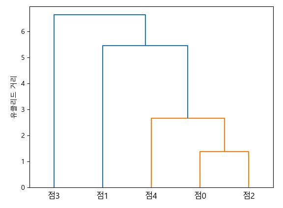
- 계층적 클러스터 분류 결과 시각화
from sklearn.cluster import AgglomerativeClustering

ac = AgglomerativeClustering(n_clusters = 3, affinity='euclidean', linkage='ward')
labels = ac.fit_predict(x)
print('결과 :', labels) # 결과 : [0 2 0 1 0]
from sklearn.cluster import AgglomerativeClustering
AgglomerativeClustering(n_clueters = 3, affinty='euclidean', linkage='ward') : 병합 군집 알고리즘
a = labels.reshape(-1, 1)
print(a)
'''
[[0]
 [2]
 [0]
 [1]
 [0]]
'''
x1 = np.hstack([x, a])
print('x1 :', x1)
'''
x1 :
[[6.96469186 2.86139335 0.        ]
 [2.26851454 5.51314769 2.        ]
 [7.1946897  4.2310646  0.        ]
 [9.80764198 6.84829739 1.        ]
 [4.80931901 3.92117518 0.        ]]
'''
x_0 = x1[x1[:, 2] == 0, :]
x_1 = x1[x1[:, 2] == 1, :]
x_2 = x1[x1[:, 2] == 2, :]

plt.scatter(x_0[:, 0], x_0[:, 1])
plt.scatter(x_1[:, 0], x_1[:, 1])
plt.scatter(x_2[:, 0], x_2[:, 1])
plt.legend(['cluster0', 'cluster1', 'cluster2'])
plt.show()
계층적 클러스터링 : iris
* cluster2.py
import pandas as pd
from sklearn.datasets import load_iris
import matplotlib.pyplot as plt

iris = load_iris()
iris_df = pd.DataFrame(iris.data, columns=iris.feature_names)
print(iris_df.head(3))
'''
   sepal length (cm)  sepal width (cm)  petal length (cm)  petal width (cm)
0                5.1               3.5                1.4               0.2
1                4.9               3.0                1.4               0.2
2                4.7               3.2                1.3               0.2
'''
print(iris_df.loc[0:4, ['sepal length (cm)', 'sepal width (cm)']])
'''
   sepal length (cm)  sepal width (cm)
0                5.1               3.5
1                4.9               3.0
2                4.7               3.2
3                4.6               3.1
4                5.0               3.6
'''
from scipy.spatial.distance import pdist, squareform
#dist_vec = pdist(iris_df.loc[:, ['sepal length (cm)', 'sepal width (cm)']], metric = 'euclidean')
dist_vec = pdist(iris_df.loc[0:4, ['sepal length (cm)', 'sepal width (cm)']], metric = 'euclidean')
print(dist_vec) # 데이터간 거리
# [0.53851648 0.5 0.64031242 0.14142136 0.28284271 0.31622777
# 0.60827625 0.14142136 0.5 0.64031242]row_dist = pd.DataFrame(squareform(dist_vec)) # 테이블 형태로 변경
print('row_dist :\n', row_dist)
'''
0 1 2 3 4
0 0.000000 0.538516 0.500000 0.640312 0.141421
1 0.538516 0.000000 0.282843 0.316228 0.608276
2 0.500000 0.282843 0.000000 0.141421 0.500000
3 0.640312 0.316228 0.141421 0.000000 0.640312
4 0.141421 0.608276 0.500000 0.640312 0.000000
'''from scipy.cluster.hierarchy import linkage, dendrogram
row_clusters = linkage(dist_vec, method='complete') # 응집형 계층적 군집 분석
print('row_clusters :\n', row_clusters)
'''
[[0. 4. 0.14142136 2. ]
[2. 3. 0.14142136 2. ]
[1. 6. 0.31622777 3. ]
[5. 7. 0.64031242 5. ]]
'''
df = pd.DataFrame(row_clusters, columns=['id1', 'id2', 'dist', 'count'])
print(df)
'''
   id1  id2      dist  count
0  0.0  4.0  0.141421    2.0
1  2.0  3.0  0.141421    2.0
2  1.0  6.0  0.316228    3.0
3  5.0  7.0  0.640312    5.0
'''
row_dend = dendrogram(row_clusters)  # dendrodgram
plt.ylabel('dist test')
plt.show()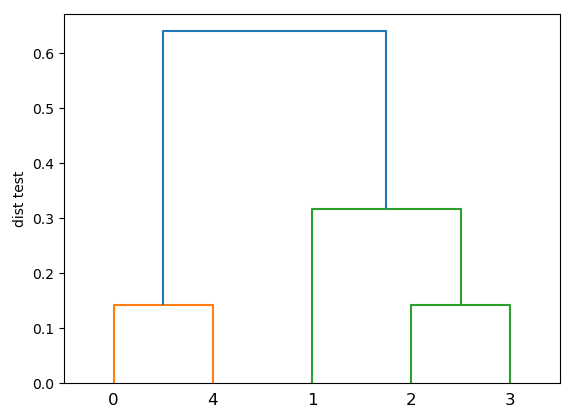
from sklearn.cluster import AgglomerativeClustering

ac = AgglomerativeClustering(n_clusters = 2, affinity='euclidean', linkage='complete')
x = iris_df.loc[0:4, ['sepal length (cm)', 'sepal width (cm)']]
labels = ac.fit_predict(x)
print('클러스터 결과 :', labels) # 결과 : [1 0 0 0 1]
plt.hist(labels)
plt.grid(True)
plt.show()
비계층적 군집분석
yganalyst.github.io/ml/ML_clustering/
[클러스터링] 비계층적(K-means, DBSCAN) 군집분석
비계층적 군집분석 방법인 K-means와 DBSCAN에 대해 알아보자
yganalyst.github.io
'BACK END > Deep Learning' 카테고리의 다른 글
| [딥러닝] DBScan (0) | 2021.03.22 |
|---|---|
| [딥러닝] k-means (0) | 2021.03.22 |
| [딥러닝] Neural Network (0) | 2021.03.19 |
| [딥러닝] KNN (0) | 2021.03.18 |
| [딥러닝] RandomForest (0) | 2021.03.17 |