RandomForest
: 앙상블 기법(여러개의 Decision Tree를 묶어 하나의 모델로 사용)
: 정량적인 분석 모델
RandomForestClassifier 분류 모델 연습
* randomForest1.py
from sklearn.ensemble import RandomForestClassifier
from sklearn.model_selection import train_test_split
import pandas as pd
from sklearn import model_selection
import numpy as np
from sklearn.metrics._scorer import accuracy_scorer

df = pd.read_csv('https://raw.githubusercontent.com/pykwon/python/master/testdata_utf8/titanic_data.csv')
print(df.head(3), df.shape) # (891, 12)
'''
   PassengerId  Survived  Pclass  ...     Fare Cabin  Embarked
0            1         0       3  ...   7.2500   NaN         S
1            2         1       1  ...  71.2833   C85         C
2            3         1       3  ...   7.9250   NaN         S
'''
print(df.columns)
# Index(['PassengerId', 'Survived', 'Pclass', 'Name', 'Sex', 'Age', 'SibSp',
#        'Parch', 'Ticket', 'Fare', 'Cabin', 'Embarked'],
#       dtype='object')
print(df.info())
 #   Column       Non-Null Count  Dtype
# ---  ------       --------------  -----
#  0   PassengerId  891 non-null    int64
#  1   Survived     891 non-null    int64
#  2   Pclass       891 non-null    int64
#  3   Name         891 non-null    object
#  4   Sex          891 non-null    object
#  5   Age          714 non-null    float64
#  6   SibSp        891 non-null    int64
#  7   Parch        891 non-null    int64
#  8   Ticket       891 non-null    object
#  9   Fare         891 non-null    float64
#  10  Cabin        204 non-null    object
#  11  Embarked     889 non-null    object

print(df.isnull().any())
# PassengerId    False
# Survived       False
# Pclass         False
# Name           False
# Sex            False
# Age             True
# SibSp          False
# Parch          False
# Ticket         False
# Fare           False
# Cabin           True
# Embarked Truedf.isnull().any() : null 값 확인.
df = df.dropna(subset=['Pclass','Age','Sex'])
print(df.head(3), df.shape) # (714, 12)

df_x = df[['Pclass','Age','Sex']]
print(df_x.head(3))
'''
   Pclass   Age     Sex
0       3  22.0    male
1       1  38.0  female
2       3  26.0  female
'''df.dropna(subset=['칼럼1', '칼럼2',..]) : 칼럼에 결측치가 있으면 제거.
from sklearn.preprocessing import LabelEncoder, OneHotEncoder

df_x.loc[:, 'Sex'] = LabelEncoder().fit_transform(df_x['Sex']) # female : 0, male : 1
df_x['Sex'] = df_x['Sex'].apply(lambda x: 1 if x=='male' else 0) # 위와 동일

print(df_x.head(3), df_x.shape) # (714, 3)
'''
   Pclass   Age  Sex
0       3  22.0    1
1       1  38.0    0
2       3  26.0    0
'''

df_y = df['Survived']
print(df_y.head(3), df_y.shape) # (714,)
'''
0    0
1    1
2    1
'''

df_x2 = pd.DataFrame(OneHotEncoder().fit_transform(df_x['Pclass'].values[:,np.newaxis]).toarray(),\
                     columns = ['f_class', 's_class', 't_class'], index=df_x.index)
print(df_x2.head(3))
'''
   f_class  s_class  t_class
0      0.0      0.0      1.0
1      1.0      0.0      0.0
2      0.0      0.0      1.0
'''

df_x = pd.concat([df_x, df_x2], axis=1)
print(df_x.head(3))
'''
   Pclass   Age  Sex  f_class  s_class  t_class
0       3  22.0    1      0.0      0.0      1.0
1       1  38.0    0      1.0      0.0      0.0
2       3  26.0    0      0.0      0.0      1.0
'''
from sklearn.preprocessing import LabelEncoder
LabelEncoder().fit_transform(df['범주형 칼럼']) : 범주형 데이터를 수치형으로 변환.
from sklearn.preprocessing import OneHotEncoder
OneHotEncoder().fit_transform(df['칼럼명']).toarray() : One hot encoding
np.newaxis : 차원 증가.
pd.concat([칼럼, .. ], axis=1) : 열 방향 합치기
# train / test
(train_x,  test_x, train_y, test_y) = train_test_split(df_x, df_y)

# model
from sklearn.metrics import accuracy_score

model = RandomForestClassifier(n_estimators=500, criterion='entropy')
fit_model = model.fit(train_x, train_y)

pred = fit_model.predict(test_x)
print('예측값:', pred[:10])           # [0 0 0 1 0 0 0 1 0 0]
print('실제값:', test_y[:10].ravel()) # [0 1 0 0 1 0 0 1 0 0]

print('acc :', sum(test_y == pred) / len(test_y))
print('acc :', accuracy_score(test_y, pred))
from sklearn.ensemble import RandomForestClassifier
RandomForestClassifier(n_estimators=100, criterion='entropy') : n_estimators : 트리 수, criterion : 분할 품질 측정 방법.
from sklearn.metrics import accuracy_score
accuracy_score(실제값, 예측값) : 정확도 산출.
ravel() : 차원 축소.
- RandomForestClassifier API
scikit-learn.org/stable/modules/generated/sklearn.ensemble.RandomForestClassifier.html
sklearn.ensemble.RandomForestClassifier — scikit-learn 0.24.1 documentation
scikit-learn.org
보스톤 지역의 주택 평균가격 예측
* randomForest_regressor.py
import pandas as pd
import matplotlib.pyplot as plt
from sklearn.datasets import load_boston

boston = load_boston()
print(boston.DESCR)
# MEDV     Median value of owner-occupied homes in $1000's

# DataFrame 값으로 변환
dfx = pd.DataFrame(boston.data, columns = boston.feature_names)
# dataset에서 독립변수 값만 추출
dfy = pd.DataFrame(boston.target, columns = ['MEDV'])
# dataset에서 종속변수 값 추출

print(dfx.head(3), dfx.shape) # (506, 13)
'''
      CRIM    ZN  INDUS  CHAS    NOX  ...  RAD    TAX  PTRATIO       B  LSTAT
0  0.00632  18.0   2.31   0.0  0.538  ...  1.0  296.0     15.3  396.90   4.98
1  0.02731   0.0   7.07   0.0  0.469  ...  2.0  242.0     17.8  396.90   9.14
2  0.02729   0.0   7.07   0.0  0.469  ...  2.0  242.0     17.8  392.83   4.03
'''
print(dfy.head(3), dfy.shape) # (506, 1)
'''
   MEDV
0  24.0
1  21.6
2  34.7
'''
df = pd.concat([dfx, dfy], axis=1)
print(df.head(3))
'''
      CRIM    ZN  INDUS  CHAS    NOX  ...    TAX  PTRATIO       B  LSTAT  MEDV
0  0.00632  18.0   2.31   0.0  0.538  ...  296.0     15.3  396.90   4.98  24.0
1  0.02731   0.0   7.07   0.0  0.469  ...  242.0     17.8  396.90   9.14  21.6
2  0.02729   0.0   7.07   0.0  0.469  ...  242.0     17.8  392.83   4.03  34.7
'''
from sklearn.datasets import load_boston
load_boston() : boston 부동산관련 dataset.
- 상관계수
pd.set_option('display.max_columns', 100) # 데이터 프레임 출력시 생략 값 출력.
print(df.corr()) # 상관계수 확인
# RM       average number of rooms per dwelling.                   상관계수 : 0.695360
# AGE      proportion of owner-occupied units built prior to 1940. 상관계수 : -0.376955
# LSTAT    % lower status of the population                        상관계수 : -0.737663
pd.set_option('display.max_columns', 100) :데이터 프레임 출력시 컬럼 생략 값 출력.
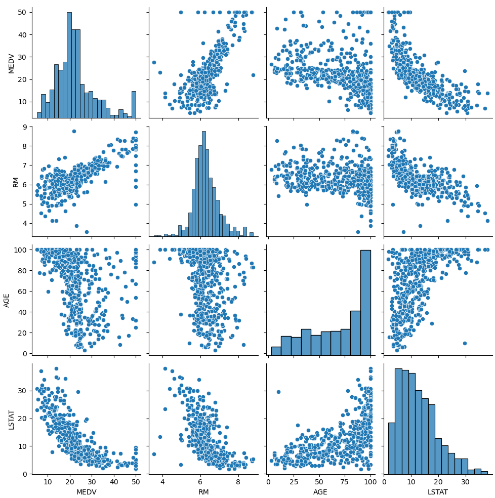
- 시각화
import seaborn as sns
cols = ['MEDV', 'RM', 'AGE', 'LSTAT']
sns.pairplot(df[cols])
plt.show()
import seaborn as sns
sns.pairplot(데이터) : 변수 간 산점 분포도 출력.
- sklearn에 맞게 데이터 변환
x = df[['LSTAT']].values # sklearn에서 득립변수는 2차원
y = df['MEDV'].values
print(x[:2])             # [[4.98] [9.14]]
print(y[:2])             # [24.  21.6]
- DecisionTreeRegressor
# 실습 1
from sklearn.tree import DecisionTreeRegressor
from sklearn.metrics import r2_score

model = DecisionTreeRegressor(max_depth=3).fit(x, y)
print('predict :', model.predict(x)[:5]) # predict : [30.47142857 25.84701493 37.315625   43.98888889 30.47142857]
print('real :', y[:5])                   # real : [24.  21.6 34.7 33.4 36.2]
r2 = r2_score(y, model.predict(x))
print('결정계수(R2, 설명력) :', r2)          # 결정계수(R2, 설명력) : 0.6993833085636556
from sklearn.tree import DecisionTreeRegressor
DecisionTreeRegressor(max_depth=).fit(x, y) : 결정 트리 회귀
from sklearn.metrics import r2_score
r2_score(실제값, 예측값) : r square 값 산출
- RandomForestRegressor
# 실습 2
from sklearn.ensemble import RandomForestRegressor

model2 = RandomForestRegressor(n_estimators=1000, criterion='mse', random_state=123).fit(x, y) # criterion='mse' 평균 제곱오차
print('predict2 :', model2.predict(x)[:5]) # predict : [24.7535     22.0408     35.2609581  38.8436     32.00298571]
print('real :', y[:5])                     # real : [24.  21.6 34.7 33.4 36.2]
r2_1 = r2_score(y, model2.predict(x))
print('결정계수(R2, 설명력) :', r2_1)          # 결정계수(R2, 설명력) : 0.9096858991691069
from sklearn.ensemble import RandomForestRegressor
RandomForestRegressor(n_estimators=, criterion='mse', random_state=).fit(x, y) : criterion='mse' 평균 제곱오차
- 학습/검정 자료로 분리
from sklearn.model_selection import train_test_split
x_train, x_test, y_train, y_test = train_test_split(x, y, test_size=0.3, random_state=123)
model2.fit(x_train, y_train)

r2_train = r2_score(y_train, model2.predict(x_train))
print('train에 대한 설명력 :', r2_train)  # train에 대한 설명력 : 0.9090659680794153

r2_test = r2_score(y_test, model2.predict(x_test))
print('test에 대한 설명력 :', r2_test)    # test에 대한 설명력 : 0.5779609792473676
# 독립변수의 수를 늘려주면 결과는 개선됨.
from sklearn.model_selection import train_test_split
train_test_split(x, y, test_size=, random_state=) : train/test로 분리
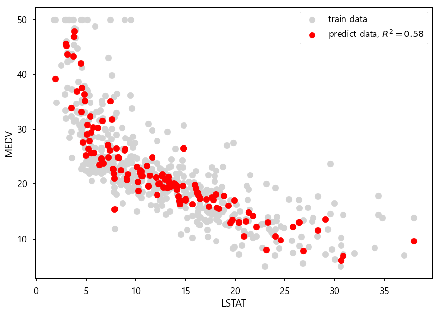
- 시각화
from matplotlib import style
style.use('seaborn-talk')
plt.scatter(x, y, c='lightgray', label='train data')
plt.scatter(x_test, model2.predict(x_test), c='r', label='predict data, $R^2=%.2f$'%r2_test)
plt.xlabel('LSTAT')
plt.ylabel('MEDV')
plt.legend()
plt.show()
from matplotlib import style
print(plt.style.available) : 사용 가능 스타일 출력.
style.use('스타일명') : matplot 스타일 사용.
- 새로운 값으로 예측
import numpy as np
print(x_test[:3])                        # [[10.11] [ 6.53] [ 3.76]]
x_new = [[50.11], [26.53], [1.76]]
print('예상 집값 :', model2.predict(x_new)) # 예상 집값 : [ 9.6527  11.0907  45.34095]
배깅 / 부스팅
배깅(Bagging) - Random Forest
: 데이터에서 여러 bootstrap 자료 생성, 모델링 후 결합하여 최종 예측 모형을 만드는 알고리즘
boostrap aggregating의 약어로 데이터를 가방(bag)에 쓸어 담아 복원 추출하여 여러 개의 표본을 만들어 이를 기반으로 각각의 모델을 개발한 후에 결과를 하나로 합쳐 하나의 모델을 만들어 내는 것이다.
배깅을 통해서 얻을 수 있는 효과는 '알고리즘의 안정성'이다.
단일 seed 하나의 값을 기준으로 데이터를 추출하여 모델을 생성해 나는 것보다, 여러 개의 다양한 표본을 사용함으로써 모델을 만드는 것이 모집단을 잘 대표할 수 있게 된다.
또한 명목형 변수 (Categorical data)의 경우 투표(voting) 방식, 혹은 가장 높은 확률값으로 예측 결과값을 합치며 연속형 변수(numeric data)의 경우에는 평균(average)으로 값을 집계한다.
또한 배깅은 병렬 처리를 사용할 수 있는데, 독립적인 데이터 셋으로 독립된 모델을 만들기 때문에 모델 생성에 있어서 매우 효율적이다.
부스팅(Boosting) - XGBoost
: 오분류 개체들에 가중치를 적용하여 새로운 분류 규칙 생성 반복 기반 최종 예측 모형 생성
좀 더 알아보자면 Boosting이란 약한 분류기를 결합하여 강한 분류기를 만드는 과정이다.
분류기 A, B, C 가 있고, 각각의 0.3 정도의 accuracy를 보여준다고 하자.
A, B, C를 결합하여 더 높은 정확도, 예를 들어 0.7 정도의 accuracy를 얻는 게 앙상블 알고리즘의 기본 원리다.
Boosting은 이 과정을 순차적으로 실행한다.
A 분류기를 만든 후, 그 정보를 바탕으로 B 분류기를 만들고, 다시 그 정보를 바탕으로 C 분류기를 만든다.
그리고 최종적으로 만들어진 분류기들을 모두 결합하여 최종 모델을 만드는 것이 Boosting의 원리다.
대표적인 알고리즘으로 에이다부스트가 있다. AdaBoost는 Adaptive Boosting의 약자이다.
Adaboost는 ensemble-based classifier의 일종으로 weak classifier를 반복적으로 적용해서, data의 특징을 찾아가는 알고리즘.
- anaconda prompt
pip install xgboost
* xgboost1.py
# RandomForest vs xgboost
import pandas as pd
from sklearn import datasets
from sklearn.model_selection import train_test_split
from sklearn.ensemble import RandomForestClassifier
from sklearn import metrics
import numpy as np
import xgboost as xgb       # pip install xgboost

if __name__ == '__main__':
    iris = datasets.load_iris()
    print('아이리스 종류 :', iris.target_names)
    print('데이터 열 이름 :', iris.feature_names)

    # iris data로 Dataframe
    data = pd.DataFrame(
        {
            'sepal length': iris.data[:, 0],
            'sepal width': iris.data[:, 1],
            'petal length': iris.data[:, 2],
            'petal width': iris.data[:, 3],
            'species': iris.target
        }
    )
    print(data.head(2))
    '''
           sepal length  sepal width  petal length  petal width  species
    0           5.1          3.5           1.4          0.2        0
    1           4.9          3.0           1.4          0.2        0
    '''

    x = data[['sepal length', 'sepal width', 'petal length', 'petal width']]
    y = data['species']

    # 테스트 데이터 30%
    x_train, x_test, y_train, y_test = train_test_split(x, y, test_size=0.3, random_state=123)

    # 학습 진행
    model = RandomForestClassifier(n_estimators=100)  # RandomForestClassifier - Bagging 방법 : 병렬 처리
    model = xgb.XGBClassifier(booster='gbtree', max_depth=4, n_estimators=100) # XGBClassifier - Boosting : 직렬처리
    # 속성 - booster: 의사결정 기반 모형(gbtree), 선형 모형(linear)
    #    - max_depth [기본값: 6]: 과적합 방지를 위해서 사용되며 CV를 사용해서 적절한 값이 제시되어야 하고 보통 3-10 사이 값이 적용된다.

    model.fit(x_train, y_train)

    # 예측
    y_pred = model.predict(x_test)
    print('예측값 : ', y_pred[:5])
    # 예측값 :  [1 2 2 1 0]

    print('실제값 : ', np.array(y_test[:5]))
    # 실제값 :  [1 2 2 1 0]

    print('정확도 : ', metrics.accuracy_score(y_test, y_pred))
    # 정확도 :  0.9333333333333333
import xgboost as xgb
xgb.XGBClassifier(booster='gbtree', max_depth=, n_estimators=) : XGBoost 분류 - Boosting(직렬처리)
booster : 의사결정 기반 모형(gbtree), 선형 모형(linear)
max_depth : 과적합 방지를 위해서 사용되며 CV를 사용해서 적절한 값이 제시되어야 하고 보통 3-10 사이 값이 적용됨.
(default: 6)
'BACK END > Deep Learning' 카테고리의 다른 글
| [딥러닝] Neural Network (0) | 2021.03.19 |
|---|---|
| [딥러닝] KNN (0) | 2021.03.18 |
| [딥러닝] Decision Tree (0) | 2021.03.17 |
| [딥러닝] 나이브 베이즈 (0) | 2021.03.17 |
| [딥러닝] PCA (0) | 2021.03.16 |