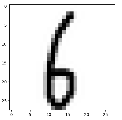
fig = plt.figure(figsize=(15, 3))
fig.subplots_adjust(hspace = 0.4, wspace = 0.4)

for i, idx in enumerate(range(len(x_test[:10]))):
    img = x_test[idx]
    ax = fig.add_subplot(1, len(x_test[:10]), i+1)
    ax.axis('off')
    ax.text(0.5, -0.35, 'pred=' + str(pred_single[idx]),\
            fontsize=10, ha = 'center', transform = ax.transAxes)
    ax.text(0.5, -0.7, 'actual=' + str(actual_single[idx]),\
            fontsize=10, ha = 'center', transform = ax.transAxes)
    ax.imshow(img)

plt.show()
- CNN + DENSE 레이어로만 분류작업2
import numpy as np
import matplotlib.pyplot as plt
from tensorflow.keras.layers import Input, Flatten, Dense, Conv2D, Activation, BatchNormalization, ReLU, LeakyReLU, MaxPool2D
from tensorflow.keras.models import Sequential, Model
from tensorflow.keras.optimizers import Adam
from tensorflow.keras.utils import to_categorical
from tensorflow.keras.datasets import cifar10
input_layer = Input(shape=(32,32,3))
x = Conv2D(filters=64, kernel_size=3, strides=2, padding='same')(input_layer)
x = MaxPool2D(pool_size=(2,2))(x)
#x = ReLU(x)
x = BatchNormalization()(x)
x = LeakyReLU()(x)

x = Conv2D(filters=64, kernel_size=3, strides=2, padding='same')(x)
x = MaxPool2D(pool_size=(2,2))(x)
x = BatchNormalization()(x)
x = LeakyReLU()(x)

x = Flatten()(x)

x = Dense(512)(x)
x = BatchNormalization()(x)
x = LeakyReLU()(x)

x = Dense(128)(x)
x = BatchNormalization()(x)
x = LeakyReLU()(x)

x = Dense(NUM_CLASSES)(x)
output_layer = Activation('softmax')(x)

model = Model(input_layer, output_layer)
import tensorflow as tf

from tensorflow.keras.models import Sequential
from tensorflow.keras.layers import Dense, Conv2D, Flatten, Dropout, MaxPooling2D
from tensorflow.keras.preprocessing.image import ImageDataGenerator

import os
import numpy as np
import matplotlib.pyplot as plt
train_dir = os.path.join(PATH, 'train')
validation_dir = os.path.join(PATH, 'validation')

train_cats_dir = os.path.join(train_dir, 'cats')  # directory with our training cat pictures
train_dogs_dir = os.path.join(train_dir, 'dogs')  # directory with our training dog pictures
validation_cats_dir = os.path.join(validation_dir, 'cats')  # directory with our validation cat pictures
validation_dogs_dir = os.path.join(validation_dir, 'dogs')  # directory with our validation dog pictures
- 이미지를 확인
num_cats_tr = len(os.listdir(train_cats_dir))
num_dogs_tr = len(os.listdir(train_dogs_dir))
# num_cats_te = len(os.listdir(test_cats_dir))
# num_dogs_te = len(os.listdir(test_dogs_dir))

num_cats_val = len(os.listdir(validation_cats_dir))
num_dogs_val = len(os.listdir(validation_dogs_dir))

total_train = num_cats_tr + num_dogs_tr
total_val = num_cats_val + num_dogs_val
# total_te = num_cats_te + num_dogs_te

print('total training cat images:', num_cats_tr)
print('total training dog images:', num_dogs_tr)
# print('total test dog images:', total_te)
# total training cat images: 1000
# total training dog images: 1000

print('total validation cat images:', num_cats_val)
print('total validation dog images:', num_dogs_val)
# total validation cat images: 500
# total validation dog images: 500
print("--")
print("Total training images:", total_train)
print("Total validation images:", total_val)
# Total training images: 2000
# Total validation images: 1000
- ImageDataGenerator
train_image_generator = ImageDataGenerator(rescale=1./255) # Generator for our training data
validation_image_generator = ImageDataGenerator(rescale=1./255) # Generator for our validation data

train_data_gen = train_image_generator.flow_from_directory(batch_size=batch_size,
                                                           directory=train_dir,
                                                           shuffle=True,
                                                           target_size=(IMG_HEIGHT, IMG_WIDTH),
                                                           class_mode='binary')
val_data_gen = validation_image_generator.flow_from_directory(batch_size=batch_size,
                                                              directory=validation_dir,
                                                              target_size=(IMG_HEIGHT, IMG_WIDTH),
                                                              class_mode='binary')
4. 데이터 확인
sample_training_images, _ = next(train_data_gen)

# This function will plot images in the form of a grid with 1 row and 5 columns where images are placed in each column.
def plotImages(images_arr):
    fig, axes = plt.subplots(1, 5, figsize=(20,20))
    axes = axes.flatten()
    for img, ax in zip( images_arr, axes):
        ax.imshow(img)
        ax.axis('off')
    plt.tight_layout()
    plt.show()

plotImages(sample_training_images[:5])
image_gen = ImageDataGenerator(rescale=1./255, horizontal_flip=True)
train_data_gen = image_gen.flow_from_directory(batch_size=batch_size,
                                               directory=train_dir,shuffle=True,
                                               target_size=(IMG_HEIGHT, IMG_WIDTH))
augmented_images = [train_data_gen[0][0][0] for i in range(5)]

# Re-use the same custom plotting f
image_gen = ImageDataGenerator(rescale=1./255, horizontal_flip=True)
train_data_gen = image_gen.flow_from_directory(batch_size=batch_size,
                                               directory=train_dir,
                                               shuffle=True,
                                               target_size=(IMG_HEIGHT, IMG_WIDTH))

augmented_images = [train_data_gen[0][0][0] for i in range(5)]

# Re-use the same custom plotting function defined and used
# above to visualize the training images
plotImages(augmented_images)
전부 적용
image_gen_train = ImageDataGenerator(
                    rescale=1./255,
                    rotation_range=45,
                    width_shift_range=.15,
                    height_shift_range=.15,
                    horizontal_flip=True,
                    zoom_range=0.5
                    )

train_data_gen = image_gen_train.flow_from_directory(batch_size=batch_size,
                                                     directory=train_dir,
                                                     shuffle=True,
                                                     target_size=(IMG_HEIGHT, IMG_WIDTH),
                                                     class_mode='binary')

augmented_images = [train_data_gen[0][0][0] for i in range(5)]
plotImages(augmented_images)
! ls -al
! pip install tensorflow-datasets
import os
import numpy as np
import matplotlib.pyplot as plt
import tensorflow as tf
import tensorflow_datasets as tfds
전이 학습 파이 튜닝 : 미리 학습된 ConvNet의 마지막 FC Layer만 변경해 분류 실행
이전 학습의 모바일넷을 동경시키고 새로 추가한 레이어만 학습 (베이스 모델의 후방 레이어 일부만 다시 학습)
먼저 베이스 모델을 동결한 후 학습 진행 -> 학습이 끝나면 동결 해제
base_model.trainable = True
print('베이스 모델의 레이어 :', len(base_model.layers)) # 베이스 모델의 레이어 : 154

fine_tune_at = 100

for layer in base_model.layers[:fine_tune_at]:
    layer.trainable = False
import tensorflow.compat.v1 as tf   # tf2.x 환경에서 1.x 소스 실행 시
tf.disable_v2_behavior()            # tf2.x 환경에서 1.x 소스 실행 시

x_data = [[1,2],[2,3],[3,4],[4,3],[3,2],[2,1]]
y_data = [[0],[0],[0],[1],[1],[1]]

# placeholders for a tensor that will be always fed.
X = tf.placeholder(tf.float32, shape=[None, 2])
Y = tf.placeholder(tf.float32, shape=[None, 1])
W = tf.Variable(tf.random_normal([2, 1]), name='weight')
b = tf.Variable(tf.random_normal([1]), name='bias')

# Hypothesis using sigmoid: tf.div(1., 1. + tf.exp(tf.matmul(X, W)))
hypothesis = tf.sigmoid(tf.matmul(X, W) + b)

# 로지스틱 회귀에서 Cost function 구하기
cost = -tf.reduce_mean(Y * tf.log(hypothesis) + (1 - Y) * tf.log(1 - hypothesis))

# Optimizer(코스트 함수의 최소값을 찾는 알고리즘) 구하기
train = tf.train.GradientDescentOptimizer(learning_rate=0.01).minimize(cost)

predicted = tf.cast(hypothesis > 0.5, dtype=tf.float32)
accuracy = tf.reduce_mean(tf.cast(tf.equal(predicted, Y), dtype=tf.float32))

with tf.Session() as sess:
    sess.run(tf.global_variables_initializer())
    for step in range(10001):
        cost_val, _ = sess.run([cost, train], feed_dict={X: x_data, Y: y_data})
        if step % 200 == 0:
            print(step, cost_val)

    # Accuracy report (정확도 출력)
    h, c, a = sess.run([hypothesis, predicted, accuracy],feed_dict={X: x_data, Y: y_data})
    print("\nHypothesis: ", h, "\nCorrect (Y): ", c, "\nAccuracy: ", a)
import tensorflow.compat.v1 as tf
tf.disable_v2_behavior() : 텐서플로우 2환경에서 1 소스 실행 시 사용
import numpy as np
from tensorflow.keras.models import Sequential
from tensorflow.keras.layers import Dense, Activation

np.random.seed(0)

x = np.array([[1,2],[2,3],[3,4],[4,3],[3,2],[2,1]])
y = np.array([[0],[0],[0],[1],[1],[1]])

model = Sequential([
    Dense(units = 1, input_dim=2),  # input_shape=(2,)
    Activation('sigmoid')
])

model.compile(loss='binary_crossentropy', optimizer='adam', metrics=['accuracy'])

model.fit(x, y, epochs=1000, batch_size=1, verbose=1)

meval = model.evaluate(x,y)
print(meval)            # [0.209698(loss),  1.0(정확도)]

pred = model.predict(np.array([[1,2],[10,5]]))
print('예측 결과 : ', pred)     # [[0.16490099] [0.9996613 ]]
print('예측 결과 : ', np.squeeze(np.where(pred > 0.5, 1, 0)))  # [0 1]

for i in pred:
    print(1 if i > 0.5 else print(0))
print([1 if i > 0.5 else 0 for i in pred])
# 2. function API 사용
from tensorflow.keras.layers import Input
from tensorflow.keras.models import Model

inputs = Input(shape=(2,))
outputs = Dense(1, activation='sigmoid')
model2 = Model(inputs, outputs)

model2.compile(loss='binary_crossentropy', optimizer='adam', metrics=['accuracy'])

model2.fit(x, y, epochs=500, batch_size=1, verbose=0)

meval2 = model2.evaluate(x,y)
print(meval2)            # [0.209698(loss),  1.0(정확도)]
# 과적합 방지 - train/test
x_train, x_test, y_train, y_test = train_test_split(x, y, test_size=0.3, random_state=12)
print(x_train.shape, x_test.shape, y_train.shape)     # (4547, 12) (1950, 12) (4547,)

# model
model = Sequential()
model.add(Dense(30, input_dim=12, activation='relu'))
model.add(tf.keras.layers.BatchNormalization()) # 배치정규화. 그래디언트 손실과 폭주 문제 개선
model.add(Dense(15, activation='relu'))
model.add(tf.keras.layers.BatchNormalization()) # 배치정규화. 그래디언트 손실과 폭주 문제 개선
model.add(Dense(8, activation='relu'))
model.add(tf.keras.layers.BatchNormalization()) # 배치정규화. 그래디언트 손실과 폭주 문제 개선
model.add(Dense(1, activation='sigmoid'))
print(model.summary()) # Total params: 992

# 학습 설정
model.compile(optimizer='adam', loss='binary_crossentropy', metrics=['accuracy'])

# 모델 평가
loss, acc = model.evaluate(x_train, y_train, verbose=2)
print('훈련되지않은 모델의 분류 정확도 :{:5.2f}%'.format(100 * acc))  # 훈련되지않은 모델의 평가 :25.14%
model.add(tf.keras.layers.BatchNormalization()) : 배치정규화. 그래디언트 손실과 폭주 문제 개선
# 모델 저장 및 폴더 설정
import os
MODEL_DIR = './model/'
if not os.path.exists(MODEL_DIR): # 폴더가 없으면 생성
    os.mkdir(MODEL_DIR)

# 모델 저장조건 설정
modelPath = "model/{epoch:02d}-{loss:4f}.hdf5"

# 모델 학습 시 모니터링의 결과를 파일로 저장
chkpoint = ModelCheckpoint(filepath='./model/abc.hdf5', monitor='loss', save_best_only=True)
#chkpoint = ModelCheckpoint(filepath=modelPath, monitor='loss', save_best_only=True)

# 학습 조기 종료
early_stop = EarlyStopping(monitor='loss', patience=5)

# 훈련
# 과적합 방지 - validation_split
history = model.fit(x_train, y_train, epochs=10000, batch_size=64,\
                    validation_split=0.3, callbacks=[early_stop, chkpoint])

model.load_weights('./model/abc.hdf5')
from tensorflow.keras.callbacks import ModelCheckpoint
checkkpoint = ModelCheckpoint(filepath=경로, monitor='loss', save_best_only=True) : 모델 학습 시 모니터링의 결과를 파일로 저장
from tensorflow.keras.callbacks import EarlyStopping
early_stop = EarlyStopping(monitor='loss', patience=5) : 학습 조기 종료
model.fit(x, y, epochs=, batch_size=, validation_split=, callbacks=[early_stop, checkpoint])
'''
여기에서는 인터넷 영화 데이터베이스(Internet Movie Database)에서 수집한 50,000개의 영화 리뷰 텍스트를 담은
IMDB 데이터셋을 사용하겠습니다. 25,000개 리뷰는 훈련용으로, 25,000개는 테스트용으로 나뉘어져 있습니다.
훈련 세트와 테스트 세트의 클래스는 균형이 잡혀 있습니다. 즉 긍정적인 리뷰와 부정적인 리뷰의 개수가 동일합니다.
매개변수 num_words=10000은 훈련 데이터에서 가장 많이 등장하는 상위 10,000개의 단어를 선택합니다.
데이터 크기를 적당하게 유지하기 위해 드물에 등장하는 단어는 제외하겠습니다.
'''

from tensorflow.keras.datasets import imdb
(train_data, train_labels), (test_data, test_labels) = imdb.load_data(num_words=10000)

print(train_data[0])   # 각 숫자는 사전에 있는 전체 문서에 나타난 모든 단어에 고유한 번호를 부여한 어휘사전
# [1, 14, 22, 16, 43, 530, 973, ...

print(train_labels) # 긍정 1 부정0
# [1 0 0 ... 0 1 0]

aa = []
for seq in train_data:
    #print(max(seq))
    aa.append(max(seq))

print(max(aa), len(aa))
# 9999 25000

word_index = imdb.get_word_index() # 단어와 정수 인덱스를 매핑한 딕셔너리
reverse_word_index = dict([(value, key) for (key, value) in word_index.items()])
decord_review = ' '.join([reverse_word_index.get(i - 3, '?') for i in train_data[0]])
print(decord_review)
# ? this film was just brilliant casting location scenery story direction ...
from tensorflow.keras import models, layers, regularizers

model = models.Sequential()
model.add(layers.Dense(16, activation='relu', input_shape=(10000, ), kernel_regularizer=regularizers.l2(0.01)))
# regularizers.l2(0.001) : 가중치 행렬의 모든 원소를 제곱하고 0.001을 곱하여 네트워크의 전체 손실에 더해진다는 의미, 이 규제(패널티)는 훈련할 때만 추가됨
model.add(layers.Dropout(0.3)) # 과적합 방지를 목적으로 노드 일부는 학습에 참여하지 않음
model.add(layers.Dense(16, activation='relu'))
model.add(layers.Dense(1, activation='sigmoid'))

model.compile(optimizer='adam', loss='binary_crossentropy', metrics=['acc'])

print(model.summary())
layers.Dropout(n) : 과적합 방지를 목적으로 노드 일부는 학습에 참여하지 않음
from tensorflow.keras import models, layers, regularizers
x_train, x_test, y_train, y_test = train_test_split(x_scaler, y, test_size=0.3, random_state=1)
n_features = x_train.shape[1] # 열
n_classes = y_train.shape[1]  # 열
print(n_features, n_classes)  # 4 3 => input, output수
- n의 개수 만큼 모델 생성 함수
from tensorflow.keras.models import Sequential
from tensorflow.keras.layers import Dense

def create_custom_model(input_dim, output_dim, out_node, n, model_name='model'):
    def create_model():
        model = Sequential(name = model_name)
        for _ in range(n): # layer 생성
            model.add(Dense(out_node, input_dim = input_dim, activation='relu'))

        model.add(Dense(output_dim, activation='softmax'))
        model.compile(optimizer='adam', loss='categorical_crossentropy', metrics=['acc'])
        return model
    return create_model # 주소 반환(클로저)
models = [create_custom_model(n_features, n_classes, 10, n, 'model_{}'.format(n)) for n in range(1, 4)]
# layer수가 2 ~ 5개 인 모델 생성

for create_model in models:
    print('-------------------------')
    create_model().summary()
    # Total params: 83
    # Total params: 193
    # Total params: 303
- train
history_dict = {}

for create_model in models: # 각 모델 loss, acc 출력
    model = create_model()
    print('Model names :', model.name)
    # 훈련
    history = model.fit(x_train, y_train, batch_size=5, epochs=50, verbose=0, validation_split=0.3)
    # 평가
    score = model.evaluate(x_test, y_test)
    print('test dataset loss', score[0])
    print('test dataset acc', score[1])
    history_dict[model.name] = [history, model]

print(history_dict)
# {'model_1': [<tensorflow.python.keras.callbacks.History object at 0x00000273BA4E7280>, <tensorflow.python.keras.engine.sequential.Sequential object at 0x00000273B9B22A90>], ...}
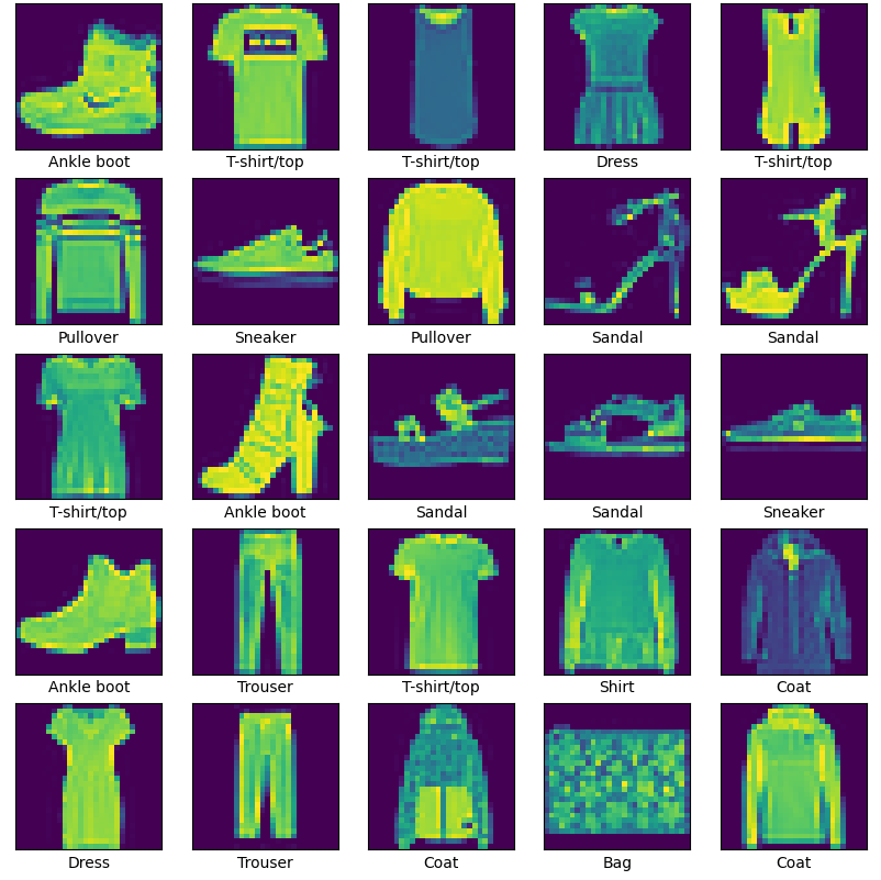
plt.figure(figsize=(10, 10))
for i in range(25):
    plt.subplot(5, 5, i+1)
    plt.xticks([])
    plt.yticks([])
    plt.xlabel(class_names[train_labels[i]])
    plt.imshow(train_image[i])

plt.show()
model.save('ke21.h5')

model = tf.keras.models.load_model('ke21.h5')

import pickle
histoy = histoy.history # loss, acc

with open('data.pickle', 'wb') as f: # 파일 저장
    pickle.dump(histoy)              # 객체 저장

with open('data.pickle', 'rb') as f: # 파일 읽기
    history = pickle.load(f)         # 객체 읽기
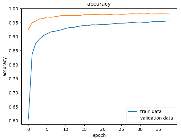
import matplotlib.pyplot as plt
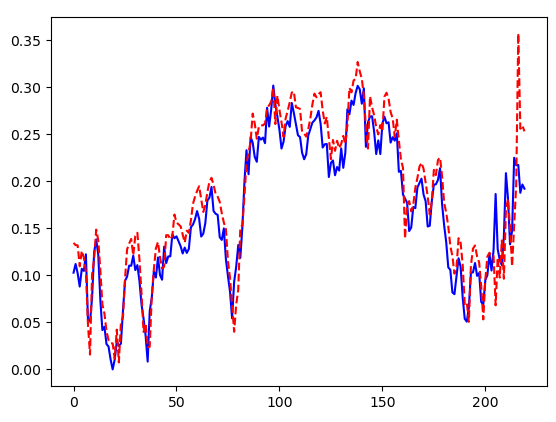
def plot_acc(title = None):
plt.plot(history['accuracy'])
plt.plot(history['val_accuracy'])
if title is not None:
plt.title(title)
plt.ylabel(title)
plt.xlabel('epoch')
plt.legend(['train data', 'validation data'], loc = 0)
plot_acc('accuracy')
plt.show()
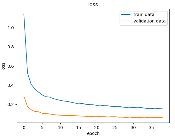
def plot_loss(title = None):
plt.plot(history['loss'])
plt.plot(history['val_loss'])
if title is not None:
plt.title(title)
plt.ylabel(title)
plt.xlabel('epoch')
plt.legend(['train data', 'validation data'], loc = 0)
plot_loss('loss')
plt.show()
import tensorflow as tf
from tensorflow.keras.datasets import mnist
from tensorflow.keras.utils import to_categorical
from tensorflow.keras.callbacks import ModelCheckpoint, EarlyStopping
import matplotlib.pyplot as plt
import numpy as np
import sys
import tensorflow as tf
import numpy as np

print(tf.keras.__version__)
1. 데이터 수집 및 가공
x = np.array([[0,0],[0,1],[1,0],[1,1]])
#y = np.array([0,1,1,1]) # or
#y = np.array([0,0,0,1]) # and
y = np.array([0,1,1,0]) # xor : node가 1인 경우 처리 불가
2. 모델 생성(네트워크 구성)
from tensorflow.keras.models import Sequential
from tensorflow.keras.layers import Dense, Activation

model = Sequential([
    Dense(input_dim =2, units=1),
    Activation('sigmoid')
    ])

model = Sequential()
model.add(Dense(units=1, input_dim=2))
model.add(Activation('sigmoid'))
# input_dim : 입력층의 뉴런 수
# units : 출력 뉴런 수
from tensorflow.keras.models import Sequential
from tensorflow.keras.layers import Dense, Activation
# 완벽한 모델이라 판단되면 모델을 저장
model.save('test.hdf5')
del model # 모델 삭제

from tensorflow.keras.models import load_model
model2 = load_model('test.hdf5')
pred2 = (model2.predict(x) > 0.5).astype('int32')
print('pred2 :\n', pred2.flatten())
model.save('파일명.hdf5') : 모델 삭제
del model : 모델 삭제
from tensorflow.keras.models import load_model model = load_model('파일명.hdf5') : 모델 불러오기
논리 게이트 XOR 해결을 위해 Node 추가
* ke2.py
import tensorflow as tf
import numpy as np

# 1. 데이터 수집 및 가공
x = np.array([[0,0],[0,1],[1,0],[1,1]])
y = np.array([0,1,1,0]) # xor : node가 1인 경우 처리 불가
# 단순 선형회귀 예측 모형 작성
# x = 5일 때 f(x) = 50에 가까워지는 w 값 찾기

import tensorflow as tf
import numpy as np

x = tf.Variable(5.0)
w = tf.Variable(0.0)
@tf.function
def train_step():
    with tf.GradientTape() as tape: # 자동 미분을 위한 API 제공
        #print(tape.watch(w))
        y = tf.multiply(w, x) + 0
        loss = tf.square(tf.subtract(y, 50)) # (예상값 - 실제값)의 제곱
    grad = tape.gradient(loss, w)  # 자동 미분
    mu = 0.01 # 학습율
    w.assign_sub(mu * grad)
    return loss

for i in range(10):
    loss = train_step()
    print('{:1}, w:{:4.3}, loss:{:4.5}'.format(i, w.numpy(), loss.numpy()))
'''
0, w: 5.0, loss:2500.0
1, w: 7.5, loss:625.0
2, w:8.75, loss:156.25
3, w:9.38, loss:39.062
4, w:9.69, loss:9.7656
5, w:9.84, loss:2.4414
6, w:9.92, loss:0.61035
7, w:9.96, loss:0.15259
8, w:9.98, loss:0.038147
9, w:9.99, loss:0.0095367
'''
tf.GradientTape() :
gradient(loss, w) : 자동미분
# 옵티마이저 객체 사용
opti = tf.keras.optimizers.SGD()

x = tf.Variable(5.0)
w = tf.Variable(0.0)

@tf.function
def train_step2():
    with tf.GradientTape() as tape:          # 자동 미분을 위한 API 제공
        y = tf.multiply(w, x) + 0
        loss = tf.square(tf.subtract(y, 50)) # (예상값 - 실제값)의 제곱
    grad = tape.gradient(loss, w)            # 자동 미분
    opti.apply_gradients([(grad, w)])
    return loss

for i in range(10):
    loss = train_step2()
    print('{:1}, w:{:4.3}, loss:{:4.5}'.format(i, w.numpy(), loss.numpy()))
opti = tf.keras.optimizers.SGD() :
opti.apply_gradients([(grad, w)]) :
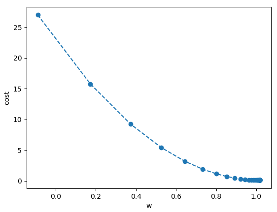
# 최적의 기울기, y절편 구하기
opti = tf.keras.optimizers.SGD()
x = tf.Variable(5.0)
w = tf.Variable(0.0)
b = tf.Variable(0.0)
@tf.function
def train_step3():
with tf.GradientTape() as tape: # 자동 미분을 위한 API 제공
#y = tf.multiply(w, x) + b
y = tf.add(tf.multiply(w, x), b)
loss = tf.square(tf.subtract(y, 50)) # (예상값 - 실제값)의 제곱
grad = tape.gradient(loss, [w, b]) # 자동 미분
opti.apply_gradients(zip(grad, [w, b]))
return loss
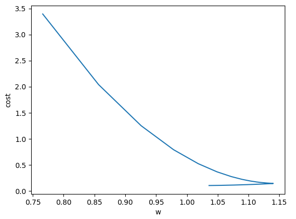
w_val = [] # 시각화 목적으로 사용
cost_val = []
for i in range(10):
loss = train_step3()
print('{:1}, w:{:4.3}, loss:{:4.5}, b:{:4.3}'.format(i, w.numpy(), loss.numpy(), b.numpy()))
w_val.append(w.numpy())
cost_val.append(loss.numpy())
'''
0, w: 5.0, loss:2500.0, b: 1.0
1, w: 7.4, loss:576.0, b:1.48
2, w:8.55, loss:132.71, b:1.71
3, w: 9.1, loss:30.576, b:1.82
4, w:9.37, loss:7.0448, b:1.87
5, w: 9.5, loss:1.6231, b: 1.9
6, w:9.56, loss:0.37397, b:1.91
7, w:9.59, loss:0.086163, b:1.92
8, w: 9.6, loss:0.019853, b:1.92
9, w:9.61, loss:0.0045738, b:1.92
'''
import matplotlib.pyplot as plt
plt.plot(w_val, cost_val, 'o')
plt.xlabel('w')
plt.ylabel('cost')
plt.show()
중앙값(median)과 IQR(interquartile range) 사용. 아웃라이어의 영향을 최소화
* ke8_scaler.py
from tensorflow.keras.models import Sequential
from tensorflow.keras.layers import Dense
from tensorflow.keras import optimizers
from tensorflow.keras.optimizers import SGD, RMSprop, Adam
import numpy as np
import pandas as pd
import matplotlib.pyplot as plt
import tensorflow as tf
from sklearn.preprocessing import MinMaxScaler, minmax_scale, StandardScaler, RobustScaler
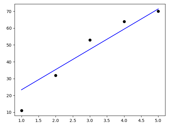
data = pd.read_csv('https://raw.githubusercontent.com/pykwon/python/master/testdata_utf8/Advertising.csv')
del data['no']
print(data.head(2))
'''
tv radio newspaper sales
0 230.1 37.8 69.2 22.1
1 44.5 39.3 45.1 10.4
'''
# 모델 생성
model = Sequential()

model.add(Dense(1, input_dim =3)) # 레이어 1개
model.add(Activation('linear'))

model.add(Dense(1, input_dim =3, activation='linear'))
print(model.summary())
tf.keras.utils.plot_model(model,'abc.png')
tf.keras.utils.plot_model(model,'파일명') : 레이어 도식화하여 파일 저장.
from tensorflow.keras.models import Sequential
from tensorflow.keras.layers import Dense
from tensorflow.keras import optimizers
import numpy as np
import pandas as pd
import matplotlib.pyplot as plt
import tensorflow as tf
from tensorflow.keras.datasets import boston_housing

#print(boston_housing.load_data())
(x_train, y_train), (x_test, y_test) = boston_housing.load_data()
print(x_train[:2], x_train.shape) # (404, 13)
print(y_train[:2], y_train.shape) # (404,)
print(x_test[:2], x_test.shape)   # (102, 13)
print(y_test[:2], y_test.shape)   # (102,)
'''
CRIM: 자치시(town) 별 1인당 범죄율
ZN: 25,000 평방피트를 초과하는 거주지역의 비율
INDUS:비소매상업지역이 점유하고 있는 토지의 비율
CHAS: 찰스강에 대한 더미변수(강의 경계에 위치한 경우는 1, 아니면 0)
NOX: 10ppm 당 농축 일산화질소
RM: 주택 1가구당 평균 방의 개수
AGE: 1940년 이전에 건축된 소유주택의 비율
DIS: 5개의 보스턴 직업센터까지의 접근성 지수
RAD: 방사형 도로까지의 접근성 지수
TAX: 10,000 달러 당 재산세율
PTRATIO: 자치시(town)별 학생/교사 비율
B: 1000(Bk-0.63)^2, 여기서 Bk는 자치시별 흑인의 비율을 말함.
LSTAT: 모집단의 하위계층의 비율(%)
MEDV: 본인 소유의 주택가격(중앙값) (단위: $1,000)
'''