Tensorflow - 이미지 분류
- ImageData
www.tensorflow.org/api_docs/python/tf/keras/preprocessing/image/ImageDataGenerator
tf.keras.preprocessing.image.ImageDataGenerator
Generate batches of tensor image data with real-time data augmentation.
www.tensorflow.org
- LeakyReLU
05-1. 심층 신경망 학습 - 활성화 함수, 가중치 초기화
5-1. 심층 신경망 학습 - 활성화 함수, 가중치 초기화 저번 포스팅 04. 인공신경망에서 예제로 살펴본 신경망은 hidden layer가 2개인 얕은 DNN에 대해 다루었다. 하지만, 모델이 복잡해질수록 hidden layer
excelsior-cjh.tistory.com
CIRAR-10
: 10개의 레이블, 6만장의 칼라 이미지(5만장 - train, 1만장 - test)
- tf_cnn_cifar10.ipynb
#airplane, automobile, bird, cat, deer, dog, frog, horse, ship, truck
# DENSE 레이어로만 분류작업1

import numpy as np
import matplotlib.pyplot as plt
from tensorflow.keras.layers import Input, Flatten, Dense, Conv2D
from tensorflow.keras.models import Sequential, Model
from tensorflow.keras.optimizers import Adam
from tensorflow.keras.utils import to_categorical
from tensorflow.keras.datasets import cifar10
NUM_CLASSES = 10
(x_train, y_train), (x_test, y_test) = cifar10.load_data()
print('train data')
print(x_train.shape) # (50000, 32, 32, 3)
print(x_train.shape[0])
print(x_train.shape[3])
print('test data')
print(x_test.shape) # (10000, 32, 32, 3)
print(x_train[0]) # [[[ 59 62 63] ...
print(y_train[0]) # [6] frog
plt.figure(figsize=(12, 4))
plt.subplot(131)
plt.imshow(x_train[0], interpolation='bicubic')
plt.subplot(132)
plt.imshow(x_train[1], interpolation='bicubic')
plt.subplot(133)
plt.imshow(x_train[2], interpolation='bicubic')
x_train = x_train.astype('float32') / 255.0
x_test = x_test.astype('float32') / 255.0

y_train = to_categorical(y_train, NUM_CLASSES)
y_test = to_categorical(y_test, NUM_CLASSES)
print(x_train[54, 12, 13, 1]) # 0.36862746
print(x_train[1,12,13,2])  # 0.59607846
- 방법 1 Sequential API 사용(CNN 사용 X)
model = Sequential([
        Dense(512, input_shape=(32, 32, 3), activation='relu'),
        Flatten(),
        Dense(128, activation='relu'),
        Dense(NUM_CLASSES, activation='softmax')
])
print(model.summary()) # Total params: 67,112,330
- 방법 2 function API 사용(CNN 사용 X)
input_layer = Input((32, 32, 3))
x = Flatten()(input_layer)
x = Dense(512, activation='relu')(x)
x = Dense(128, activation='relu')(x)
output_layer = Dense(NUM_CLASSES, activation='softmax')(x)

model = Model(input_layer, output_layer)
print(model.summary()) # Total params: 1,640,330
- train
opt = Adam(lr=0.01)
model.compile(loss='categorical_crossentropy', optimizer=opt, metrics=['accuracy'])
model.fit(x_train, y_train, batch_size=128, epochs=10, shuffle=True, verbose=2)
print('acc : %.4f'%(model.evaluate(x_test, y_test, batch_size=128)[1]))  # acc : 0.1000
print('loss : %.4f'%(model.evaluate(x_test, y_test, batch_size=128)[0])) # loss : 2.3030
CLASSES = np.array(['airplane', 'automobile', 'bird', 'cat', 'deer', 'dog', 'frog', 'horse', 'ship', 'truck'])

pred = model.predict(x_test[:10])
pred_single = CLASSES[np.argmax(pred, axis = -1)]
actual_single = CLASSES[np.argmax(y_test[:10], axis = -1)]
print('예측값 :', pred_single)
# 예측값 : ['frog' 'frog' 'frog' 'frog' 'frog' 'frog' 'frog' 'frog' 'frog' 'frog']
print('실제값 :', actual_single)
# 실제값 : ['cat' 'ship' 'ship' 'airplane' 'frog' 'frog' 'automobile' 'frog' 'cat' 'automobile']
print('분류 실패 수 :', (pred_single != actual_single).sum())
# 분류 실패 수 : 7
- 시각화
fig = plt.figure(figsize=(15, 3))
fig.subplots_adjust(hspace = 0.4, wspace = 0.4)

for i, idx in enumerate(range(len(x_test[:10]))):
    img = x_test[idx]
    ax = fig.add_subplot(1, len(x_test[:10]), i+1)
    ax.axis('off')
    ax.text(0.5, -0.35, 'pred=' + str(pred_single[idx]),\
            fontsize=10, ha = 'center', transform = ax.transAxes)
    ax.text(0.5, -0.7, 'actual=' + str(actual_single[idx]),\
            fontsize=10, ha = 'center', transform = ax.transAxes)
    ax.imshow(img)

plt.show()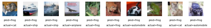
- CNN + DENSE 레이어로만 분류작업2
import numpy as np
import matplotlib.pyplot as plt
from tensorflow.keras.layers import Input, Flatten, Dense, Conv2D, Activation, BatchNormalization, ReLU, LeakyReLU, MaxPool2D
from tensorflow.keras.models import Sequential, Model
from tensorflow.keras.optimizers import Adam
from tensorflow.keras.utils import to_categorical
from tensorflow.keras.datasets import cifar10
NUM_CLASSES = 10
(x_train, y_train), (x_test, y_test) = cifar10.load_data()
x_train = x_train.astype('float32') / 255.0
x_test = x_test.astype('float32') / 255.0
y_train = to_categorical(y_train, NUM_CLASSES)
y_test = to_categorical(y_test, NUM_CLASSES)
- function API : CNN + DENSE
input_layer = Input(shape=(32,32,3))
conv_layer1 = Conv2D(filters=64, kernel_size=3, strides=2, padding='same')(input_layer)
conv_layer2 = Conv2D(filters=64, kernel_size=3, strides=2, padding='same')(conv_layer1)

flatten_layer = Flatten()(conv_layer2)

output_layer = Dense(units=10, activation='softmax')(flatten_layer)
model = Model(input_layer,  output_layer)
print(model.summary()) # Total params: 79,690
input_layer = Input(shape=(32,32,3))
x = Conv2D(filters=64, kernel_size=3, strides=2, padding='same')(input_layer)
x = MaxPool2D(pool_size=(2,2))(x)
#x = ReLU(x)
x = BatchNormalization()(x)
x = LeakyReLU()(x)
x = Conv2D(filters=64, kernel_size=3, strides=2, padding='same')(x)
x = MaxPool2D(pool_size=(2,2))(x)
x = BatchNormalization()(x)
x = LeakyReLU()(x)
x = Flatten()(x)
x = Dense(512)(x)
x = BatchNormalization()(x)
x = LeakyReLU()(x)
x = Dense(128)(x)
x = BatchNormalization()(x)
x = LeakyReLU()(x)
x = Dense(NUM_CLASSES)(x)
output_layer = Activation('softmax')(x)
model = Model(input_layer, output_layer)
- train
opt = Adam(lr=0.01)
model.compile(loss='categorical_crossentropy', optimizer=opt, metrics=['accuracy'])
model.fit(x_train, y_train, batch_size=128, epochs=10, shuffle=True, verbose=2)
print('acc : %.4f'%(model.evaluate(x_test, y_test, batch_size=128)[1]))  # acc : 0.5986
print('loss : %.4f'%(model.evaluate(x_test, y_test, batch_size=128)[0])) # loss : 1.3376
Tensor : image process, CNN
Daum 카페
cafe.daum.net
CNN을 이용하여Tensor : image process, CNN 고차원적인 이미지 분류
https://wiserloner.tistory.com/1046?category=837669
텐서플로 2.0 공홈 탐방 (cat and dog image classification)
- 이번에는 CNN을 이용하여 조금 더 고차원적인 이미지 분류를 해보겠습니다. - 과연 머신이 영상을 보고 이것이 개인지 고양이인지를 분류해낼수 있을까요? 딥러닝, 그중에 CNN을 사용하면 놀랍
wiserloner.tistory.com
- tf_cnn_dogcat.ipynb
1. 라이브러리 임포트
import tensorflow as tf

from tensorflow.keras.models import Sequential
from tensorflow.keras.layers import Dense, Conv2D, Flatten, Dropout, MaxPooling2D
from tensorflow.keras.preprocessing.image import ImageDataGenerator

import os
import numpy as np
import matplotlib.pyplot as plt
2. 데이터 다운로드
_URL = 'https://storage.googleapis.com/mledu-datasets/cats_and_dogs_filtered.zip'
path_to_zip = tf.keras.utils.get_file('cats_and_dogs.zip', origin=_URL, extract=True)
PATH = os.path.join(os.path.dirname(path_to_zip), 'cats_and_dogs_filtered')

batch_size = 128
epochs = 15
IMG_HEIGHT = 150
IMG_WIDTH = 150
3. 데이터 준비
train_dir = os.path.join(PATH, 'train')
validation_dir = os.path.join(PATH, 'validation')

train_cats_dir = os.path.join(train_dir, 'cats')  # directory with our training cat pictures
train_dogs_dir = os.path.join(train_dir, 'dogs')  # directory with our training dog pictures
validation_cats_dir = os.path.join(validation_dir, 'cats')  # directory with our validation cat pictures
validation_dogs_dir = os.path.join(validation_dir, 'dogs')  # directory with our validation dog pictures
- 이미지를 확인
num_cats_tr = len(os.listdir(train_cats_dir))
num_dogs_tr = len(os.listdir(train_dogs_dir))
# num_cats_te = len(os.listdir(test_cats_dir))
# num_dogs_te = len(os.listdir(test_dogs_dir))

num_cats_val = len(os.listdir(validation_cats_dir))
num_dogs_val = len(os.listdir(validation_dogs_dir))

total_train = num_cats_tr + num_dogs_tr
total_val = num_cats_val + num_dogs_val
# total_te = num_cats_te + num_dogs_te

print('total training cat images:', num_cats_tr)
print('total training dog images:', num_dogs_tr)
# print('total test dog images:', total_te)
# total training cat images: 1000
# total training dog images: 1000

print('total validation cat images:', num_cats_val)
print('total validation dog images:', num_dogs_val)
# total validation cat images: 500
# total validation dog images: 500
print("--")
print("Total training images:", total_train)
print("Total validation images:", total_val)
# Total training images: 2000
# Total validation images: 1000
- ImageDataGenerator
train_image_generator = ImageDataGenerator(rescale=1./255) # Generator for our training data
validation_image_generator = ImageDataGenerator(rescale=1./255) # Generator for our validation data

train_data_gen = train_image_generator.flow_from_directory(batch_size=batch_size,
                                                           directory=train_dir,
                                                           shuffle=True,
                                                           target_size=(IMG_HEIGHT, IMG_WIDTH),
                                                           class_mode='binary')
val_data_gen = validation_image_generator.flow_from_directory(batch_size=batch_size,
                                                              directory=validation_dir,
                                                              target_size=(IMG_HEIGHT, IMG_WIDTH),
                                                              class_mode='binary')
4. 데이터 확인
sample_training_images, _ = next(train_data_gen)

# This function will plot images in the form of a grid with 1 row and 5 columns where images are placed in each column.
def plotImages(images_arr):
    fig, axes = plt.subplots(1, 5, figsize=(20,20))
    axes = axes.flatten()
    for img, ax in zip( images_arr, axes):
        ax.imshow(img)
        ax.axis('off')
    plt.tight_layout()
    plt.show()

plotImages(sample_training_images[:5])
5. 모델 생성
model = Sequential([
    Conv2D(16, 3, padding='same', activation='relu', input_shape=(IMG_HEIGHT, IMG_WIDTH ,3)),
    MaxPooling2D(),
    Conv2D(32, 3, padding='same', activation='relu'),
    MaxPooling2D(),
    Conv2D(64, 3, padding='same', activation='relu'),
    MaxPooling2D(),
    Flatten(),
    Dense(512, activation='relu'),
    # Dense(1)
    Dense(1, activation='sigmoid')
])
6. 모델 컴파일
model.compile(optimizer='adam',
              loss=tf.keras.losses.BinaryCrossentropy(from_logits=True),
              metrics=['accuracy'])
7. 모델 확인
model.summary() # Total params: 10,641,441
8. 학습
history = model.fit_generator(
    train_data_gen,
    steps_per_epoch=total_train // batch_size,
    epochs=epochs,
    validation_data=val_data_gen,
    validation_steps=total_val // batch_size
)
9. 학습 결과 시각화
acc = history.history['accuracy']
val_acc = history.history['val_accuracy']

loss=history.history['loss']
val_loss=history.history['val_loss']

epochs_range = range(epochs)

plt.figure(figsize=(8, 8))
plt.subplot(1, 2, 1)
plt.plot(epochs_range, acc, label='Training Accuracy')
plt.plot(epochs_range, val_acc, label='Validation Accuracy')
plt.legend(loc='lower right')
plt.title('Training and Validation Accuracy')

plt.subplot(1, 2, 2)
plt.plot(epochs_range, loss, label='Training Loss')
plt.plot(epochs_range, val_loss, label='Validation Loss')
plt.legend(loc='upper right')
plt.title('Training and Validation Loss')
plt.show()

오버피팅 처리 오버피팅 처리
image_gen = ImageDataGenerator(rescale=1./255, horizontal_flip=True)
train_data_gen = image_gen.flow_from_directory(batch_size=batch_size,
                                               directory=train_dir,shuffle=True,
                                               target_size=(IMG_HEIGHT, IMG_WIDTH))
augmented_images = [train_data_gen[0][0][0] for i in range(5)]

# Re-use the same custom plotting f
image_gen = ImageDataGenerator(rescale=1./255, horizontal_flip=True)
train_data_gen = image_gen.flow_from_directory(batch_size=batch_size,
                                               directory=train_dir,
                                               shuffle=True,
                                               target_size=(IMG_HEIGHT, IMG_WIDTH))

augmented_images = [train_data_gen[0][0][0] for i in range(5)]

# Re-use the same custom plotting function defined and used
# above to visualize the training images
plotImages(augmented_images)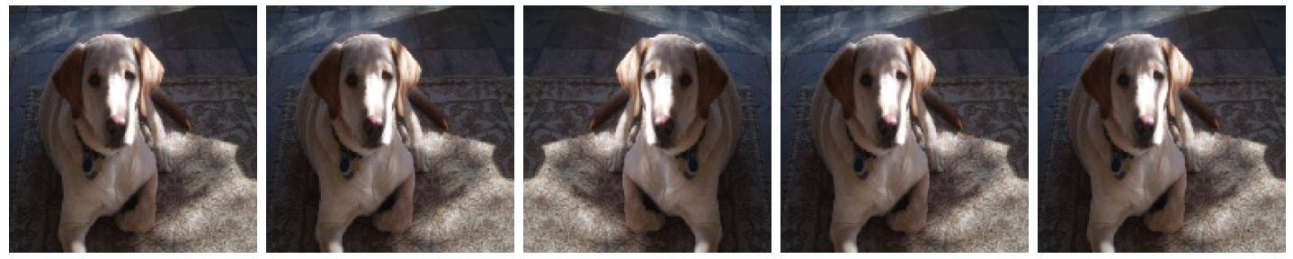
전부 적용
image_gen_train = ImageDataGenerator(
                    rescale=1./255,
                    rotation_range=45,
                    width_shift_range=.15,
                    height_shift_range=.15,
                    horizontal_flip=True,
                    zoom_range=0.5
                    )

train_data_gen = image_gen_train.flow_from_directory(batch_size=batch_size,
                                                     directory=train_dir,
                                                     shuffle=True,
                                                     target_size=(IMG_HEIGHT, IMG_WIDTH),
                                                     class_mode='binary')

augmented_images = [train_data_gen[0][0][0] for i in range(5)]
plotImages(augmented_images)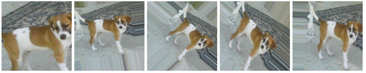
image_gen_val = ImageDataGenerator(rescale=1./255)

val_data_gen = image_gen_val.flow_from_directory(batch_size=batch_size,
                                                 directory=validation_dir,
                                                 target_size=(IMG_HEIGHT, IMG_WIDTH),
                                                 class_mode='binary')

model_new = Sequential([
    Conv2D(16, 3, padding='same', activation='relu',
           input_shape=(IMG_HEIGHT, IMG_WIDTH ,3)),
    MaxPooling2D(),
    Dropout(0.2),
    Conv2D(32, 3, padding='same', activation='relu'),
    MaxPooling2D(),
    Conv2D(64, 3, padding='same', activation='relu'),
    MaxPooling2D(),
    Dropout(0.2),
    Flatten(),
    Dense(512, activation='relu'),
    Dense(1)
])

model_new.compile(optimizer='adam',
                  loss=tf.keras.losses.BinaryCrossentropy(from_logits=True),
                  metrics=['accuracy'])

model_new.summary() # Total params: 10,641,441
11. 학습 및 확인
history = model_new.fit_generator(
    train_data_gen,
    steps_per_epoch=total_train // batch_size,
    epochs=epochs,
    validation_data=val_data_gen,
    validation_steps=total_val // batch_size
)
acc = history.history['accuracy']
val_acc = history.history['val_accuracy']

loss = history.history['loss']
val_loss = history.history['val_loss']

epochs_range = range(epochs)

plt.figure(figsize=(8, 8))
plt.subplot(1, 2, 1)
plt.plot(epochs_range, acc, label='Training Accuracy')
plt.plot(epochs_range, val_acc, label='Validation Accuracy')
plt.legend(loc='lower right')
plt.title('Training and Validation Accuracy')

plt.subplot(1, 2, 2)
plt.plot(epochs_range, loss, label='Training Loss')
plt.plot(epochs_range, val_loss, label='Validation Loss')
plt.legend(loc='upper right')
plt.title('Training and Validation Loss')
plt.show()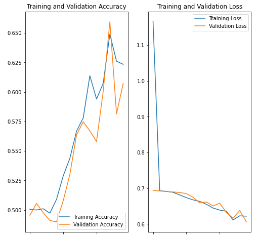
Transfer Learning(전이 학습)
: 부족한 데이터로 모델 생성시 성능이 약한 모델이 생성된다. 이에 전문회사에서 제공하는 모델을 사용하여 성능을 높인다.(모델을 라이브러리 처럼 사용)
: 미리 학습된 모델을 사용하여 내가 분류하고자 하는 데이터를 이용해 약간의 학습으로 성능 좋은 이미지 분류 모델을 얻을 수 있다.
이미지 분류 모형
cafe.daum.net/flowlife/S2Ul/31
Daum 카페
cafe.daum.net
Transfer Learning
cafe.daum.net/flowlife/S2Ul/32
Daum 카페
cafe.daum.net
* tf_cnn_trans_learn.ipynb
! ls -al
! pip install tensorflow-datasets
import os
import numpy as np
import matplotlib.pyplot as plt
import tensorflow as tf
import tensorflow_datasets as tfds
tfds.disable_progress_bar()

(raw_train, raw_validation, raw_test), metadata = tfds.load('cats_vs_dogs',
                            split = ['train[:80%]', 'train[80%:90%]', 'train[90%:]'], with_info=True, as_supervised=True)

print(raw_train)
print(raw_validation)
print(raw_test)

print(metadata)
<PrefetchDataset shapes: ((None, None, 3), ()), types: (tf.uint8, tf.int64)>
<PrefetchDataset shapes: ((None, None, 3), ()), types: (tf.uint8, tf.int64)>
<PrefetchDataset shapes: ((None, None, 3), ()), types: (tf.uint8, tf.int64)>
tfds.core.DatasetInfo(
name='cats_vs_dogs',
version=4.0.0,
description='A large set of images of cats and dogs.There are 1738 corrupted images that are dropped.',
homepage='https://www.microsoft.com/en-us/download/details.aspx?id=54765',
features=FeaturesDict({
'image': Image(shape=(None, None, 3), dtype=tf.uint8),
'image/filename': Text(shape=(), dtype=tf.string),
'label': ClassLabel(shape=(), dtype=tf.int64, num_classes=2),
}),
total_num_examples=23262,
splits={
'train': 23262,
},
supervised_keys=('image', 'label'),
citation="""@Inproceedings (Conference){asirra-a-captcha-that-exploits-interest-aligned-manual-image-categorization,
author = {Elson, Jeremy and Douceur, John (JD) and Howell, Jon and Saul, Jared},
title = {Asirra: A CAPTCHA that Exploits Interest-Aligned Manual Image Categorization},
booktitle = {Proceedings of 14th ACM Conference on Computer and Communications Security (CCS)},
year = {2007},
month = {October},
publisher = {Association for Computing Machinery, Inc.},
url = {https://www.microsoft.com/en-us/research/publication/asirra-a-captcha-that-exploits-interest-aligned-manual-image-categorization/},
edition = {Proceedings of 14th ACM Conference on Computer and Communications Security (CCS)},
}""",
redistribution_info=,
)get_label_name = metadata.features['label'].int2str
print(get_label_name)
for image, label in raw_train.take(2):
plt.figure()
plt.imshow(image)
plt.title(get_label_name(label))
plt.show()
IMG_SIZE = 160   # All images will be resized to 160 by160

def format_example(image, label):
    image = tf.cast(image, tf.float32)
    image = (image/127.5) - 1
    image = tf.image.resize(image, (IMG_SIZE, IMG_SIZE))
    return image, label

train = raw_train.map(format_example)
validation = raw_validation.map(format_example)
test = raw_test.map(format_example)

# 4. 이미지 셔플링 배칭
BATCH_SIZE = 32
SHUFFLE_BUFFER_SIZE = 1000

train_batches = train.shuffle(SHUFFLE_BUFFER_SIZE).batch(BATCH_SIZE)
validation_batches = validation.batch(BATCH_SIZE)
test_batches = test.batch(BATCH_SIZE)
# 학습 데이터는 임의로 셔플하고 배치 크기를 정하여 배치로 나누어준다.

for image_batch, label_batch in train_batches.take(1):
    pass

print(image_batch.shape)    # [32, 160, 160, 3]

# 5. 베이스 모델 생성 : 전이학습에서 사용할 베이스 모델은 Google에서 개발한 MobileNet V2 모델 사용.
IMG_SHAPE = (IMG_SIZE, IMG_SIZE, 3)

# Create the base model from the pre-trained model MobileNet V2
base_model = tf.keras.applications.MobileNetV2(input_shape=IMG_SHAPE, include_top=False, weights='imagenet')

feature_batch = base_model(image_batch)
print(feature_batch.shape)   # (32, 5, 5, 1280)

# include_top=False : 입력층 -> CNN 계층 -> 특징 추출 -> 완전 연결층
- 계층 동결
base_model.trainable = False # MobileNet V2 학습 정지
print(base_model.summary()) # Total params: 2,257,984
- 전이 학습을 위한 모델 생성
global_average_layer = tf.keras.layers.GlobalAveragePooling2D() # 급격히 feature의 수를 줄여주는 역할
feature_batch_average = global_average_layer(feature_batch)
print(feature_batch_average) # (32, 1280)

prediction_layer = tf.keras.layers.Dense(1)
prediction_batch = prediction_layer(feature_batch_average)
print(prediction_batch)      # (32, 1)

model = tf.keras.Sequential([
        base_model,
        global_average_layer,
        prediction_layer
])

base_learning_rate = 0.0001
model.compile(optimizer=tf.keras.optimizers.RMSprop(lr=base_learning_rate),\
              loss = tf.keras.losses.BinaryCrossentropy(from_logits=True), metrics=['accuracy'])
print(model.summary())
'''
Layer (type)                 Output Shape              Param #
=================================================================
mobilenetv2_1.00_160 (Functi (None, 5, 5, 1280)        2257984
_________________________________________________________________
global_average_pooling2d_3 ( (None, 1280)              0
_________________________________________________________________
dense_2 (Dense)              (None, 1)                 1281
=================================================================
Total params: 2,259,265
'''
- 현재 모델 확인
validation_steps = 20
loss0, accuracy0 = model.evaluate(validation_batches, steps=validation_steps)
print('initial loss : {:.2f}'.format(loss0))    # initial loss : 0.92
print('initial acc : {:.2f}'.format(accuracy0)) # initial acc : 0.35
- 모델 학습
initial_epochs = 5 # 10
history = model.fit(train_batches, epochs=initial_epochs, validation_data =validation_batches)
- 학습 시각화
acc = history.history['accuracy']
val_acc = history.history['val_accuracy']
loss = history.history['loss']
val_loss = history.history['val_loss']

plt.figure(figsize=(8, 8))
plt.subplot(2,1,1)
plt.plot(acc, label ='Train accuracy')
plt.plot(val_acc, label ='Validation accuracy')
plt.legend(loc='lower right')
plt.ylabel('Accuracy')
plt.ylim([min(plt.ylim()), 1])
plt.title('Training and Validation Accuracy')

plt.subplot(2,1,2)
plt.plot(loss, label ='Train losss')
plt.plot(val_loss, label ='Validation loss')
plt.legend(loc='upper right')
plt.ylabel('Cross entropy')
plt.ylim([0, 1.0])
plt.title('Training and Validation Loss')
plt.xlabel('epochs')
plt.show()
전이 학습 파이 튜닝 : 미리 학습된 ConvNet의 마지막 FC Layer만 변경해 분류 실행
이전 학습의 모바일넷을 동경시키고 새로 추가한 레이어만 학습 (베이스 모델의 후방 레이어 일부만 다시 학습)
먼저 베이스 모델을 동결한 후 학습 진행 -> 학습이 끝나면 동결 해제
base_model.trainable = True
print('베이스 모델의 레이어 :', len(base_model.layers)) # 베이스 모델의 레이어 : 154

fine_tune_at = 100

for layer in base_model.layers[:fine_tune_at]:
    layer.trainable = False
model.compile(loss = tf.keras.losses.BinaryCrossentropy(from_logits= True),\
optimizer = tf.keras.optimizers.RMSprop(lr=base_learning_rate / 10), metrics=['accuracy'])
print(model.summary()) # Total params: 2,259,265
# 파일 튜인 학습
fine_tune_epochs = 2
initial_epochs = 5
total_epochs = initial_epochs + fine_tune_epochs
history_fine = model.fit(train_batches, epochs = total_epochs, initial_epoch=history.epoch[-1],\
validation_data = validation_batches)- 시각화
print(history_fine.history)
acc += history_fine.history['accuracy']
val_acc += history_fine.history['val_accuracy']
loss += history_fine.history['loss']
val_loss += history_fine.history['val_loss']

plt.figure(figsize=(8, 8))
plt.subplot(2,1,1)
plt.plot(acc, label ='Train accuracy')
plt.plot(val_acc, label ='Validation accuracy')
plt.legend(loc='lower right')
plt.plot([initial_epochs -1, initial_epochs -1], plt.ylim(), label='Start fine tuning')
plt.ylabel('Accuracy')
plt.ylim([0.8, 1])
plt.title('Training and Validation Accuracy')

plt.subplot(2,1,2)
plt.plot(loss, label ='Train losss')
plt.plot(val_loss, label ='Validation loss')
plt.legend(loc='upper right')
plt.plot([initial_epochs -1, initial_epochs -1], plt.ylim(), label='Start fine tuning')
plt.ylabel('Cross entropy')
plt.ylim([0, 1.0])
plt.title('Training and Validation Loss')
plt.xlabel('epochs')
plt.show()
ANN, RNN(LSTM, GRU)
cafe.daum.net/flowlife/S2Ul/12
Daum 카페
cafe.daum.net
RNN
[AI] RNN, LSTM이란?
RNN(Recurrent Neural Networks)은 다른 신경망과 어떻게 다른가?RNN은 이름에서 알 수 있는 것처...
blog.naver.com
RNN (순환신경망)
: 시계열 데이터 처리 - 자연어, 번역, 이미지 캡션, 채팅, 주식 ...
from tensorflow.keras.models import Sequential
from tensorflow.keras.layers import SimpleRNN, LSTMSimpleRNN(3, input_shape =) :
LSTM(3, input_shape =) :
model = Sequential()
model.add(SimpleRNN(3, input_shape = (2, 10)))             # Total params: 42
model.add(SimpleRNN(3, input_length = 2, input_dim = 10))
model.add(LSTM(3, input_shape = (2, 10)))                   # Total params: 168

print(model.summary())
model = Sequential()
#model.add(SimpleRNN(3, batch_input_shape = (8, 2, 10))) # batch_size : 8, sequence : 2, 입력수 : 10, 출력 수 : 3
# Total params: 42
model.add(LSTM(3, batch_input_shape = (8, 2, 10))) # Total params: 168
print(model.summary())model = Sequential()
#model.add(SimpleRNN(3, batch_input_shape = (8, 2, 10), return_sequences=True))
model.add(LSTM(3, batch_input_shape = (8, 2, 10), return_sequences=True))
print(model.summary())
- SimpleRNN
www.tensorflow.org/api_docs/python/tf/keras/layers/SimpleRNN
tf.keras.layers.SimpleRNN | TensorFlow Core v2.4.1
Fully-connected RNN where the output is to be fed back to input.
www.tensorflow.org
- LSTM
www.tensorflow.org/api_docs/python/tf/keras/layers/LSTM
tf.keras.layers.LSTM | TensorFlow Core v2.4.1
Long Short-Term Memory layer - Hochreiter 1997.
www.tensorflow.org
'BACK END > Deep Learning' 카테고리의 다른 글
| [딥러닝] GAN (0) | 2021.04.12 |
|---|---|
| [딥러닝] RNN, NLP (0) | 2021.04.05 |
| [딥러닝] Keras - Logistic (0) | 2021.03.25 |
| [딥러닝] Keras - Linear (0) | 2021.03.23 |
| [딥러닝] TensorFlow (0) | 2021.03.22 |