[코딩] Circle Square

순환신경망 (Recurrent Neueal Network, RNN)

: 시퀀스 단위의 입력을 시퀀스 단위의 출력으로 처리하는 모델

: 시계열 데이터 처리 - 자연어, 번역, 이미지 캡션, 채팅, 주식 ...

: LSTM, GRU, ..

 - RNN

wikidocs.net/22886

* tf_rnn.ipynb

from tensorflow.keras.models import Sequential
from tensorflow.keras.layers import SimpleRNN, LSTM

model = Sequential()

model.add(SimpleRNN(3, input_shape = (2, 10)))
#model.add(SimpleRNN(3, input_length = 2, input_dim = 10))

print(model.summary())                # Total params: 42

from tensorflow.keras.layers. import SimpleRNN

SimpleRNN(a, batch_input_shape = (b, c, d)) :  출력 수(a), batch_size(b), sequence(c), 입력수(d)

model = Sequential()

model.add(LSTM(3, input_shape = (2, 10)))

print(model.summary())                # Total params: 168

from tensorflow.keras.layers. import LSTM

LSTM(a, batch_input_shape = (b, c, d)) : 출력 수(a), batch_size(b), sequence(c), 입력수(d)

model = Sequential()

model.add(SimpleRNN(3, batch_input_shape = (8, 2, 10)))
# batch_size : 8, sequence : 2, 입력수 : 10, 출력 수 : 3

print(model.summary())                # Total params: 42

model = Sequential()

model.add(LSTM(3, batch_input_shape = (8, 2, 10)))

print(model.summary())                # Total params: 168

model = Sequential()

model.add(SimpleRNN(3, batch_input_shape = (8, 2, 10), return_sequences=True))

print(model.summary())                # Total params: 42

model = Sequential()

model.add(LSTM(3, batch_input_shape = (8, 2, 10), return_sequences=True))

print(model.summary())               # Total params: 168

NLP(자연어 처리)

자연어 : 순차적

문장 -> 단어/문자열/형태소/자소(자음/모음) -> code화(숫자) -> one -hot encoding or word2vec(단어간 관계 예측) -> embeding처리

4개의 숫자를 통해 그 다음 숫자를 예측하는 RNN 모델 생성

 * tf_rnn2.ipynb

import tensorflow as tf
import numpy as np

x = []
y = []
for i in range(6):              # 0 ~ 5
    lst = list(range(i, i + 4)) # 0 ~ 3, 1 ~ 4, 2 ~ 5 ...
    print(lst)
    x.append(list(map(lambda c:[c / 10], lst)))
    y.append((i + 4) /10)

print(x)
# [[[0.0], [0.1], [0.2], [0.3]], [[0.1], [0.2], [0.3], [0.4]], [[0.2], [0.3], [0.4], [0.5]], [[0.3], [0.4], [0.5], [0.6]], [[0.4], [0.5], [0.6], [0.7]], [[0.5], [0.6], [0.7], [0.8]]]
print(y)
# [0.4, 0.5, 0.6, 0.7, 0.8, 0.9]

x = np.array(x)
y = np.array(y)

for i in range(len(x)): # 0 ~ 5
    print(x[i], y[i])
# [[0. ]
#  [0.1]
#  [0.2]
#  [0.3]] 0.4
# [[0.1]
#  [0.2]
#  [0.3]
#  [0.4]] 0.5
# ...

model = tf.keras.Sequential([
    #tf.keras.layers.SimpleRNN(units=10, activation='tanh', input_shape=[4, 1]),  # Total params: 131
    #tf.keras.layers.LSTM(units=10, activation='tanh', input_shape=[4, 1]),       # Total params: 491
    tf.keras.layers.GRU(units=10, activation='tanh', input_shape=[4, 1]),         # Total params: 401

    tf.keras.layers.Dense(1)
])

model.compile(optimizer='adam', loss='mse')
print(model.summary())

model.fit(x, y, epochs=100, verbose=0)
print('예측값 :', model.predict(x))
# 예측값 : [[0.380357  ]
#  [0.50256383]
#  [0.6151931 ]
#  [0.7163592 ]
#  [0.8050702 ]
#  [0.88109314]]
print('실제값 :', y)
# 실제값 : [0.4 0.5 0.6 0.7 0.8 0.9]
print()

print(model.predict(np.array([[[0.6], [0.7], [0.9]]])))
# [[0.76507646]]
print(model.predict(np.array([[[-0.1], [0.2], [0.4], [0.9]]])))
# [[0.6791251]]

Dimension for RNN

 : RNN모형을 구현할 때 핵심이 되는 데이터 구조

 : many-to-many, many-to-one, one-to-many

 * tf_rnn3.ipynb

import numpy as np
import tensorflow as tf
from tensorflow import keras

# many-to-one
x = np.array([[[1], [2], [3]], [[2], [3], [4]], [[3], [4], [5]]], dtype=np.float32)
y = np.array([[4], [5], [6]])
print(x.shape, y.shape) # (3, 3, 1) (3, 1)

# function API 사용
layer_input = keras.Input(shape=(3, 1))
layer_rnn = keras.layers.SimpleRNN(100, activation='tanh')(layer_input)
layer_output = keras.layers.Dense(1)(layer_rnn)

model = keras.Model(layer_input, layer_output)
model.compile(loss = 'mse', optimizer='adam')
model._name = 'many-to-one'
print(model.summary())
# Layer (type)                 Output Shape              Param #   
# =================================================================
# input_2 (InputLayer)         [(None, 3, 1)]            0         
# _________________________________________________________________
# simple_rnn_1 (SimpleRNN)     (None, 100)               10200     
# _________________________________________________________________
# dense_1 (Dense)              (None, 1)                 101       
# =================================================================
# Total params: 10,301
model.fit(x, y, epochs=100, batch_size=1, verbose=1)
print('pred :', model.predict(x).flatten())
# pred : [3.902048  5.1808596 5.8828716]
print('real :', y.flatten())
# real : [4 5 6]

# many-to-many
x = np.array([[[1], [2], [3]], [[2], [3], [4]], [[3], [4], [5]]], dtype=np.float32)
y = np.array([[4], [5], [6]])
print(x.shape, y.shape) # (3, 3, 1) (3, 1)

# function API 사용
layer_input = keras.Input(shape=(3, 1))
layer_rnn = keras.layers.SimpleRNN(100, activation='tanh', return_sequences=True)(layer_input)
layer_output = keras.layers.TimeDistributed(keras.layers.Dense(1))(layer_rnn)

model = keras.Model(layer_input, layer_output)
model.compile(loss = 'mse', optimizer='adam')
model._name = 'many-to-many'
print(model.summary())
# Layer (type)                 Output Shape              Param #   
# =================================================================
# input_5 (InputLayer)         [(None, 3, 1)]            0         
# _________________________________________________________________
# simple_rnn_4 (SimpleRNN)     (None, 3, 100)            10200     
# _________________________________________________________________
# dense_4 (Dense)              (None, 3, 1)              101       
# =================================================================
# Total params: 10,301
model.fit(x, y, epochs=100, batch_size=1, verbose=1)
print('pred :', model.predict(x).flatten())
# pred : [3.429767  3.9655545 4.002289  5.02977   5.0609956 4.999564  6.3015547 5.9251485 6.001438 ]

print('real :', y.flatten())
# real : [4 5 6]

SimpleRNN(100, activation='tanh', return_sequences=True)

TimeDistributed(Dense(1))

# stacked many-to-one
x = np.array([[[1], [2], [3]], [[2], [3], [4]], [[3], [4], [5]]], dtype=np.float32)
y = np.array([[4], [5], [6]])
print(x.shape, y.shape) # (3, 3, 1) (3, 1)

# function API 사용
layer_input = keras.Input(shape=(3, 1))
layer_rnn1 = keras.layers.SimpleRNN(100, activation='tanh', return_sequences=True)(layer_input)
layer_rnn2 = keras.layers.SimpleRNN(100, activation='tanh', return_sequences=True)(layer_rnn1)
layer_output = keras.layers.Dense(1)(layer_rnn2)

model = keras.Model(layer_input, layer_output)
model.compile(loss = 'mse', optimizer='adam')
model._name = 'stacked-many-to-many'
print(model.summary())
# Layer (type)                 Output Shape              Param #   
# =================================================================
# input_8 (InputLayer)         [(None, 3, 1)]            0         
# _________________________________________________________________
# simple_rnn_8 (SimpleRNN)     (None, 3, 100)            10200     
# _________________________________________________________________
# simple_rnn_9 (SimpleRNN)     (None, 3, 100)            20100     
# _________________________________________________________________
# dense_7 (Dense)              (None, 3, 1)              101       
# =================================================================
# Total params: 30,401
model.fit(x, y, epochs=100, batch_size=1, verbose=1)
print('pred :', model.predict(x).flatten())
# pred : [3.6705296 3.9618802 3.9781656 5.160208  5.0984097 5.0837207 6.031624 5.93854   5.9503284]

print('real :', y.flatten())
# real : [4 5 6]

 - 자연어 처리

wikidocs.net/book/2155

 - 한국어 불용어

www.ranks.nl/stopwords/korean

문자열 토큰화 + LSTM 감성분류

 * tf_rnn4.ipynb

# token, corpus, vocabulary, one-hot, word2vec, tfidf,

from tensorflow.keras.preprocessing.text import Tokenizer

samples = ['The cat say on the mat.', 'The dog ate my homework.'] # list type

# token 처리 1 - word index
token_index = {}
for sam in samples:
    for word in sam.split(sep=' '):
        if word not in token_index:
            #print(word)
            token_index[word] = len(token_index)
print(token_index)
# {'The': 0, 'cat': 1, 'say': 2, 'on': 3, 'the': 4, 'mat.': 5, 'dog': 6, 'ate': 7, 'my': 8, 'homework.': 9}

print()
# token 처리 2 - word index
# tokenizer = Tokenizer(num_words=3) # num_words=3 빈도가 높은 3개의 토큰 만 작업에 참여
tokenizer = Tokenizer()
tokenizer.fit_on_texts(samples)
token_seq = tokenizer.texts_to_sequences(samples)   # 문자열을 index로 표현
print(token_seq)
# [[1, 2, 3, 4, 1, 5], [1, 6, 7, 8, 9]]
print(tokenizer.word_index)                        # 특수 문자 제거 및 대문자를 소문자로 변환
# {'the': 1, 'cat': 2, 'say': 3, 'on': 4, 'mat': 5, 'dog': 6, 'ate': 7, 'my': 8, 'homework': 9}

from tensorflow.keras.preprocessing.text import Tokenizer

 - Tokenizer API

www.tensorflow.org/api_docs/python/tf/keras/preprocessing/text/Tokenizer

tokenizer = Tokenizer(num_words=3) : num_words=3 빈도가 높은 3개의 토큰 만 작업에 참여

token_seq = tokenizer.texts_to_sequences(samples)

tokenizer.fit_on_texts(data) : 

tokenizer.word_index : 

token_mat = tokenizer.texts_to_matrix(samples, mode='binary')    # 있으면 1 없으면 0
# token_mat = tokenizer.texts_to_matrix(samples, mode='freq')      # 빈도수로 표현
# token_mat = tokenizer.texts_to_matrix(samples, mode='tfidf')   # 단어의 중요정도를 가중치로 표현
# token_mat = tokenizer.texts_to_matrix(samples, mode='count')
print(token_mat)
# [[0. 2. 1. 1. 1. 1. 0. 0. 0. 0.]
#  [0. 1. 0. 0. 0. 0. 1. 1. 1. 1.]]

# [[0.         0.86490296 0.69314718 0.69314718 0.69314718 0.69314718
#   0.         0.         0.         0.        ]
#  [0.         0.51082562 0.         0.         0.         0.
#   0.69314718 0.69314718 0.69314718 0.69314718]]

# [[0.         0.33333333 0.16666667 0.16666667 0.16666667 0.16666667
#   0.         0.         0.         0.        ]
#  [0.         0.2        0.         0.         0.         0.
#   0.2        0.2        0.2        0.2       ]]

# [[0. 1. 1. 1. 1. 1. 0. 0. 0. 0.]
#  [0. 1. 0. 0. 0. 0. 1. 1. 1. 1.]]

print(tokenizer.word_counts)
# OrderedDict([('the', 3), ('cat', 1), ('say', 1), ('on', 1), ('mat', 1), ('dog', 1), ('ate', 1), ('my', 1), ('homework', 1)])
print(tokenizer.document_count)  # 2
print(tokenizer.word_docs)
# defaultdict(<class 'int'>, {'the': 2, 'on': 1, 'cat': 1, 'mat': 1, 'say': 1, 'my': 1, 'ate': 1, 'dog': 1, 'homework': 1})

from tensorflow.keras.utils import to_categorical
token_seq = to_categorical(token_seq[0], num_classes=6)
print(token_seq)
# [[0. 1. 0. 0. 0. 0.]
#  [0. 0. 1. 0. 0. 0.]
#  [0. 0. 0. 1. 0. 0.]
#  [0. 0. 0. 0. 1. 0.]
#  [0. 1. 0. 0. 0. 0.]
#  [0. 0. 0. 0. 0. 1.]]

 - 영화 리뷰 자료로 간단한 감성분석

import numpy as np
docs = ['너무 재밌어요', '또 보고 싶어요', '참 잘 만든 영화네요', '친구에게 추천할래요', '배우가 멋져요',\
        '별로예요', '지루하고 재미없어요', '연기가 어색해요', '재미없어요', '돈 아까워요']
classes = np.array([1,1,1,1,1,0,0,0,0,0])

token = Tokenizer()
token.fit_on_texts(docs)
print(token.word_index)
# {'재미없어요': 1, '너무': 2, '재밌어요': 3, '또': 4, '보고': 5, '싶어요': 6, '참': 7, '잘': 8, '만든': 9, '영화네요': 10, '친구에게': 11,
# '추천할래요': 12, '배우가': 13, '멋져요': 14, '별로예요': 15, '지루하고': 16, '연기가': 17, '어색해요': 18, '돈': 19, '아까워요': 20}

x = token.texts_to_sequences(docs)
print('토큰화 결과 :', x)
# 토큰화 결과 : [[2, 3], [4, 5, 6], [7, 8, 9, 10], [11, 12], [13, 14], [15], [16, 1], [17, 18], [1], [19, 20]]

from tensorflow.keras.preprocessing.sequence import pad_sequences
padded_x = pad_sequences(x, 4) # 패딩 : 서로 다른 길이의 데이터를 가장 긴 데이터의 길이로 맞춘다.
# 병렬 연산을 위해서 여러 문장의 길이를 임의로 동일하게 맞춰주는 작업이 필요
print(padded_x)
# [[ 0  0  2  3]
#  [ 0  4  5  6]
#  [ 7  8  9 10]
#  [ 0  0 11 12]
#  [ 0  0 13 14]
#  [ 0  0  0 15]
#  [ 0  0 16  1]
#  [ 0  0 17 18]
#  [ 0  0  0  1]
#  [ 0  0 19 20]]

# 모델
word_size = len(token.word_index) + 1
print(word_size) # 22

from tensorflow.keras.models import Sequential
from tensorflow.keras.layers import Dense, Flatten, Embedding, LSTM
model = Sequential()
model.add(Embedding(word_size, output_dim=8, input_length=4)) # model.add(Embedding(vocabulary, output_dim, input_length))
model.add(LSTM(32, activation='tanh'))
model.add(Flatten()) # FC Layer
model.add(Dense(32, activation='relu'))
model.add(Dense(1, activation='sigmoid'))

model.compile(optimizer='adam', loss='binary_crossentropy', metrics=['accuracy'])
model.fit(padded_x, classes, epochs=10, verbose=1)
print('acc :', model.evaluate(padded_x, classes)[1])
# acc : 1.0
print('pred :', model.predict(padded_x).flatten())
# pred : [0.50115323 0.5027714  0.5044522  0.5016046  0.50048715 0.49916682  0.4971649  0.49867162 0.49731275 0.4972709 ]
print('real :', classes)
# real : [1 1 1 1 1 0 0 0 0 0]

RNN을 이용한 텍스트 생성

 : 모델이 문맥을 학습한 후 텍스트를 작성

 * tf_rnn5_token.ipynb

from tensorflow.keras.preprocessing.text import Tokenizer

text = """운동장에 눈이 많이 쌓여 있다
그 사람의 눈이 빛난다
맑은 눈이 사람 마음을 곱게 만든다"""

tok = Tokenizer()
tok.fit_on_texts([text])
encoded = tok.texts_to_sequences([text])
print(encoded)
# [[2, 1, 3, 4, 5, 6, 7, 1, 8, 9, 1, 10, 11, 12, 13]]
print(tok.word_index)
# {'눈이': 1, '운동장에': 2, '많이': 3, '쌓여': 4, '있다': 5, '그': 6, '사람의': 7, '빛난다': 8, '맑은': 9, '사람': 10, '마음을': 11, '곱게': 12, '만든다': 13}

vocab_size = len(tok.word_index) + 1
print('단어 집합의 크기 :%d'%vocab_size)
# 단어 집합의 크기 :14

sequences = list()   # feature
for line in text.split('\n'):
    encoded = tok.texts_to_sequences([line])[0]
    #print(encoded)
    # [2, 1, 3, 4, 5]
    # [6, 7, 1, 8]
    # [9, 1, 10, 11, 12, 13]
    for i in range(1, len(encoded)):
        sequ = encoded[:i + 1]
        #print(sequ)
        # [2, 1]
        # [2, 1, 3]
        # [2, 1, 3, 4]
        # [2, 1, 3, 4, 5]
        # [6, 7]
        # [6, 7, 1]
        # [6, 7, 1, 8]
        # [9, 1]
        # [9, 1, 10]
        # [9, 1, 10, 11]
        # [9, 1, 10, 11, 12]
        # [9, 1, 10, 11, 12, 13]
        sequences.append(sequ)
print(sequences)
# [[2, 1], [2, 1, 3], [2, 1, 3, 4], [2, 1, 3, 4, 5], [6, 7], [6, 7, 1], [6, 7, 1, 8], [9, 1], [9, 1, 10], [9, 1, 10, 11], [9, 1, 10, 11, 12], [9, 1, 10, 11, 12, 13]]

print('학습에 참여할 샘플 수 :', len(sequences)) # 12
print(max(len(i) for i in sequences)) # 6

# padding
from tensorflow.keras.preprocessing.sequence import pad_sequences
max_len = max(len(i) for i in sequences)
psequences = pad_sequences(sequences, maxlen = max_len, padding='pre')
# psequences = pad_sequences(sequences, maxlen = max_len, padding='post')
print(psequences)
# [[ 0  0  0  0  2  1]
#  [ 0  0  0  2  1  3]
#  [ 0  0  2  1  3  4]
#  [ 0  2  1  3  4  5]
#  [ 0  0  0  0  6  7]
#  [ 0  0  0  6  7  1]
#  [ 0  0  6  7  1  8]
#  [ 0  0  0  0  9  1]
#  [ 0  0  0  9  1 10]
#  [ 0  0  9  1 10 11]
#  [ 0  9  1 10 11 12]
#  [ 9  1 10 11 12 13]]

import numpy as np
psequences = np.array(psequences)
x = psequences[:, :-1] # feature
y = psequences[:, -1]  # label
print(x)
# [[ 0  0  0  0  2]
#  [ 0  0  0  2  1]
#  [ 0  0  2  1  3]
#  [ 0  2  1  3  4]
#  [ 0  0  0  0  6]
#  [ 0  0  0  6  7]
#  [ 0  0  6  7  1]
#  [ 0  0  0  0  9]
#  [ 0  0  0  9  1]
#  [ 0  0  9  1 10]
#  [ 0  9  1 10 11]
#  [ 9  1 10 11 12]]
print(y)
# [ 1  3  4  5  7  1  8  1 10 11 12 13]
from tensorflow.keras.utils import to_categorical
y = to_categorical(y, num_classes = vocab_size)
print(y)
# [[0. 1. 0. 0. 0. 0. 0. 0. 0. 0. 0. 0. 0. 0.]
#  [0. 0. 0. 1. 0. 0. 0. 0. 0. 0. 0. 0. 0. 0.]
#  [0. 0. 0. 0. 1. 0. 0. 0. 0. 0. 0. 0. 0. 0.]
#  [0. 0. 0. 0. 0. 1. 0. 0. 0. 0. 0. 0. 0. 0.]
#  [0. 0. 0. 0. 0. 0. 0. 1. 0. 0. 0. 0. 0. 0.]
#  [0. 1. 0. 0. 0. 0. 0. 0. 0. 0. 0. 0. 0. 0.]
#  [0. 0. 0. 0. 0. 0. 0. 0. 1. 0. 0. 0. 0. 0.]
#  [0. 1. 0. 0. 0. 0. 0. 0. 0. 0. 0. 0. 0. 0.]
#  [0. 0. 0. 0. 0. 0. 0. 0. 0. 0. 1. 0. 0. 0.]
#  [0. 0. 0. 0. 0. 0. 0. 0. 0. 0. 0. 1. 0. 0.]
#  [0. 0. 0. 0. 0. 0. 0. 0. 0. 0. 0. 0. 1. 0.]
#  [0. 0. 0. 0. 0. 0. 0. 0. 0. 0. 0. 0. 0. 1.]]

# model
from tensorflow.keras.layers import Embedding, Dense, SimpleRNN, LSTM, Flatten
from tensorflow.keras.models import Sequential

model = Sequential()
model.add(Embedding(vocab_size, 32, input_length=max_len - 1))
model.add(LSTM(32, activation='tanh'))
model.add(Flatten())
model.add(Dense(32, activation='relu'))
model.add(Dense(vocab_size, activation='softmax'))

model.compile(loss = 'categorical_crossentropy', optimizer='adam', metrics=['accuracy'])
print(model.summary())        # Total params: 10,286
model.fit(x, y, epochs=200, verbose=2)
print(model.evaluate(x, y))   # [0.07081326842308044, 1.0]

def sentence_gen(model, t, current_word, n):
    init_word = current_word
    sentence = ''
    for _ in range(n):
        encoded = t.texts_to_sequences([current_word])[0]
        encoded = pad_sequences([encoded], maxlen = max_len - 1, padding = 'pre')
        result = np.argmax(model.predict(encoded))
        # print(result)
        for word, index in t.word_index.items():
            #print('word:', word, ', index:', index)
            # word: 눈이 , index: 1
            # word: 운동장에 , index: 2
            # word: 많이 , index: 3
            # word: 쌓여 , index: 4
            # word: 있다 , index: 5
            # word: 그 , index: 6
            # word: 사람의 , index: 7
            # word: 빛난다 , index: 8
            # word: 맑은 , index: 9
            # word: 사람 , index: 10
            # word: 마음을 , index: 11
            # word: 곱게 , index: 12
            # word: 만든다 , index: 13
            if index == result:
                break
        current_word = current_word + ' ' + word
        sentence = sentence + ' '  + word # 예측단어를 문장에 저장
    sentence = init_word + sentence
    return sentence


print(sentence_gen(model, tok, '운동장에', 1))
print(sentence_gen(model, tok, '운동장에', 3))
print(sentence_gen(model, tok, '맑은', 1))
print(sentence_gen(model, tok, '맑은', 2))
print(sentence_gen(model, tok, '맑은', 3))
print(sentence_gen(model, tok, '한국', 3))
print(sentence_gen(model, tok, '파이썬', 5))
# 운동장에 눈이
# 운동장에 눈이 많이 쌓여
# 맑은 눈이
# 맑은 눈이 사람
# 맑은 눈이 사람 마음을
# 한국 눈이 눈이 사람

소설을 학습하여 새로운 소설생성

 * tf_rnn6_토지소설.ipynb

 - RNN 관련

cafe.daum.net/flowlife/S2Ul/33

import numpy as np
import random, sys
import tensorflow as tf

f = open("rnn_test_toji.txt", 'r', encoding="utf-8")
text = f.read()
#print(text)
f.close();

print('텍스트 행 수: ', len(text))  # 306967
print(set(text))  # set 집합형 함수를 이용해 중복 제거{'얻', '턴', '옮', '쩐', '제', '평',...

chars = sorted(list(set(text)))     # 중복이 제거된 문자를 하나하나 읽어 들여 정렬 
print(chars)                        # ['\n', ' ', '!', ... , '0', '1', ... 'a', 'c', 'f', '...
print('사용되고 있는 문자 수:', len(chars))   # 1469

char_indices = dict((c, i) for i, c in enumerate(chars)) # 문자와 ID
indices_char = dict((i, c) for i, c in enumerate(chars)) # ID와 문자
print(char_indices)            # ... '것': 106, '겄': 107, '겅': 108,...
print(indices_char)            # ... 106: '것', 107: '겄', 108: '겅',...

# 텍스트를 maxlen개의 문자로 자르고 다음에 오는 문자 등록하기
maxlen = 20
step = 3
sentences = []
next_chars = []

for i in range(0, len(text) - maxlen, step):
    #print(text[i: i + maxlen])
    sentences.append(text[i: i + maxlen])
    next_chars.append(text[i + maxlen])

print('학습할 구문 수:', len(sentences))        # 102316

print('텍스트를 ID 벡터로 변환')
X = np.zeros((len(sentences), maxlen, len(chars)), dtype=np.bool)
y = np.zeros((len(sentences), len(chars)), dtype=np.bool)
print(X[:3])
print(y[:3])

for i, sent in enumerate(sentences):
    #print(sent)
    for t, char in enumerate(sent):
        #print(t, ' ', char)
        X[i, t, char_indices[char]] = 1
    y[i, char_indices[next_chars[i]]] = 1

print(X[:5])  # 찾은 글자에만 True, 나머지는 False 기억
print(y[:5])

# 모델 구축하기(LSTM(RNN의 개량종)) -------------
# 하나의 LSTM 층과 그 뒤에 Dense 분류층 추가
model = tf.keras.Sequential()
model.add(tf.keras.layers.LSTM(128, activation='tanh', input_shape=(maxlen, len(chars))))

model.add(tf.keras.layers.Dense(128))
model.add(tf.keras.layers.Activation('relu'))
model.add(tf.keras.layers.Dense(len(chars)))
model.add(tf.keras.layers.Activation('softmax'))

opti = tf.keras.optimizers.Adam(lr=0.001)
model.compile(loss='categorical_crossentropy', optimizer=opti, metrics=['acc'])

from tensorflow.keras.callbacks import EarlyStopping

es = EarlyStopping(patience = 5, monitor='loss')
model.fit(X, y, epochs=500, batch_size=64, verbose=2, callbacks=[es])

print(model.evaluate(X, y))
# 확률적 샘플링 처리 함수(무작위적으로 샘플링하기 위함)
# 모델의 예측이 주어졌을 때 새로운 글자를 샘플링 
def sample_func(preds, variety=1.0):        # 후보를 배열에서 꺼내기
    # array():복사본, asarray():참조본 생성 - 원본 변경시 복사본은 변경X 참조본은 변경O
    preds = np.asarray(preds).astype('float64') 
    preds = np.log(preds) / variety         # 로그확률 벡터식을 코딩
    exp_preds = np.exp(preds)               # 자연상수 얻기
    preds = exp_preds / np.sum(exp_preds)   # softmax 공식 참조
    probas = np.random.multinomial(1, preds, 1)  # 다항식분포로 샘플 얻기
    return np.argmax(probas)

for num in range(1, 2):   # 학습시키고 텍스트 생성하기 반복    1, 60
    print()
    print('--' * 30)
    print('반복 =', num)

    # 데이터에서 한 번만 반복해서 모델 학습
    model.fit(X, y, batch_size=128, epochs=1, verbose=0) 

    # 임의의 시작 텍스트 선택하기
    start_index = random.randint(0, len(text) - maxlen - 1)

    for variety in [0.2, 0.5, 1.0, 1.2]:     # 다양한 문장 생성
        print('\n--- 다양성 = ', variety)    # 다양성 = 0.2 -> 다양성 =  0.5 -> ...
        generated = ''
        sentence = text[start_index: start_index + maxlen]
        generated += sentence
        print('--- 시드 = "' + sentence + '"')  # --- 시드 = "께 간뎅이가 부어서, 시부릴기력 있거"...
        sys.stdout.write(generated)

        # 시드를 기반으로 텍스트 자동 생성. 시드 텍스트에서 시작해서 500개의 글자를 생성
        for i in range(500):
            x = np.zeros((1, maxlen, len(chars))) # 지금까지 생성된 글자를 원핫인코딩 처리

            for t, char in enumerate(sentence):
                x[0, t, char_indices[char]] = 1.

            # 다음에 올 문자를 예측하기(다음 글자를 샘플링)
            preds = model.predict(x, verbose=0)[0]
            next_index = sample_func(preds, variety)    # 다양한 문장 생성을 위함
            next_char = indices_char[next_index]

            # 출력하기
            generated += next_char
            sentence = sentence[1:] + next_char
            sys.stdout.write(next_char)
            sys.stdout.flush()
        print()

 - Google colab

cafe.daum.net/flowlife/S2Ul/24

 - 리눅스 기본 명령어

cafe.daum.net/flowlife/9A8Q/161

 - 가상환경 tool

vmware

virtual box

 - telnet 와 ssh의 차이

m.blog.naver.com/PostView.nhn?blogId=ahnsh09&logNo=40171391492&proxyReferer=https:%2F%2Fwww.google.com%2F

뉴욕타임즈 기사의 일부 자료로 RNN 학습 모델을 만들어 기사 생성하기

 * tf_rnn7_뉴욕타임즈기사.ipynb

import pandas as pd
df = pd.read_csv('https://raw.githubusercontent.com/pykwon/python/master/testdata_utf8/articlesapril.csv')
print(df.head())
print(df.count)
print(df.columns)
# Index(['articleID', 'articleWordCount', 'byline', 'documentType', 'headline', 'keywords', 'multimedia', 
#'newDesk', 'printPage', 'pubDate','sectionName', 'snippet', 'source', 'typeOfMaterial', 'webURL'], dtype='object')

print(len(df.columns)) # 15

print(df['headline'].head())
# 0    Former N.F.L. Cheerleaders’ Settlement Offer: ...
# 1    E.P.A. to Unveil a New Rule. Its Effect: Less ...
# 2                              The New Noma, Explained
# 3                                              Unknown
# 4                                              Unknown
print(df.headline.values)
# ['Former N.F.L. Cheerleaders’ Settlement Offer: $1 and a Meeting With Goodell'
#  'E.P.A. to Unveil a New Rule. Its Effect: Less Science in Policymaking.'
#  'The New Noma, Explained' ...
#  'Gen. Michael Hayden Has One Regret: Russia'
#  'There Is Nothin’ Like a Tune' 'Unknown']

headline = []
headline.extend(list(df.headline.values))
print(headline[:10])
# ['Former N.F.L. Cheerleaders’ Settlement Offer: $1 and a Meeting With Goodell',
# 'E.P.A. to Unveil a New Rule. Its Effect: Less Science in Policymaking.', 'The New Noma, Explained', 'Unknown', 'Unknown', 'Unknown', 'Unknown', 'Unknown', 'How a Bag of Texas Dirt  Became a Times Tradition', 'Is School a Place for Self-Expression?']

# Unknown 값은 노이즈로 판단해 제거
print(len(headline)) # 1324
headline = [n for n in headline if n != 'Unknown']
print(len(headline)) # 1214

# 구굿점 제거, 소문자 처리
print('He하이llo 가a나b123다'.encode('ascii', errors="ignore").decode()) # Hello ab123
from string import punctuation
print(", python.'".strip(punctuation))                                   #  python
print(", py thon.'".strip(punctuation + ' '))                            # py thon
#-------------------------------------------------------------------

def repre_func(s):
    s = s.encode('utf8').decode('ascii', 'ignore')
    return ''.join(c for c in s if c not in punctuation).lower()

text = [repre_func(s) for s in headline]
print(text[:10])
# ['former nfl cheerleaders settlement offer 1 and a meeting with goodell', 'epa to unveil a new rule its effect less science in policymaking', 'the new noma explained', 'how a bag of texas dirt  became a times tradition', 'is school a place for selfexpression', 'commuter reprogramming', 'ford changed leaders looking for a lift its still looking', 'romney failed to win at utah convention but few believe hes doomed', 'chain reaction', 'he forced the vatican to investigate sex abuse now hes meeting with pope francis']

a.extend(b) : a에 b의 각 원소를 추가.

a.encode('ascii', errors="ignore").decode() : a에서 영문/숫자 아닌값 무시하여 제거.

from string import punctuation

a.strip(punctuation) : 구둣점 제거

 - 단어 집합 생성

from keras_preprocessing.text import Tokenizer
tok = Tokenizer()
tok.fit_on_texts(text)
print(tok.word_index)
# {'the': 1, 'a': 2, 'to': 3, 'of': 4, 'in': 5, 'for': 6, 'and': 7,  ...

vocab_size = len(tok.word_index) + 1
print('vocab_size :', vocab_size)   # 3494

sequences = list()
for line in text:
    enc = tok.texts_to_sequences([line])[0]
    for i in range(1, len(enc)):
        se = enc[:i + 1]
        sequences.append(se)

print(sequences[:11])
# [[99, 269], [99, 269, 371], [99, 269, 371, 1115], [99, 269, 371, 1115, 582], [99, 269, 371, 1115, 582, 52], [99, 269, 371, 1115, 582, 52, 7], [99, 269, 371, 1115, 582, 52, 7, 2], [99, 269, 371, 1115, 582, 52, 7, 2, 372], [99, 269, 371, 1115, 582, 52, 7, 2, 372, 10], [99, 269, 371, 1115, 582, 52, 7, 2, 372, 10, 1116], [100, 3]]

index_to_word = {}
for key, value in tok.word_index.items():
    index_to_word[value] = key
print(index_to_word)
# {1: 'the', 2: 'a', 3: 'to', 4: 'of', 5: 'in', 6: 'for', 7: 'and', ...
print(index_to_word[150])       # fire

max_len = max(len(i) for i in sequences)
print('max_len :', max_len)     # 24

from tensorflow.keras.preprocessing.sequence import pad_sequences
sequences = pad_sequences(sequences, maxlen = max_len, padding = 'pre')
print(sequences[:3])
# [[   0    0    0    0    0    0    0    0    0    0    0    0    0    0     0    0    0    0    0    0    0    0   99  269]
#  [   0    0    0    0    0    0    0    0    0    0    0    0    0    0     0    0    0    0    0    0    0   99  269  371]
#  [   0    0    0    0    0    0    0    0    0    0    0    0    0    0     0    0    0    0    0    0   99  269  371 1115]]

import numpy as np
sequences = np.array(sequences)
x = sequences[:, :-1] # feature
y = sequences[:, -1]  # label
print(x[:3])
# [[  0   0   0   0   0   0   0   0   0   0   0   0   0   0   0   0   0   0    0   0   0   0  99]
#  [  0   0   0   0   0   0   0   0   0   0   0   0   0   0   0   0   0   0    0   0   0  99 269]
#  [  0   0   0   0   0   0   0   0   0   0   0   0   0   0   0   0   0   0    0   0  99 269 371]]

print(y[:3])
# [ 269  371 1115]

from tensorflow.keras.utils import to_categorical
y = to_categorical(y, num_classes=vocab_size)
print(y[0])
# [0. 0. 0. ... 0. 0. 0.]

from tensorflow.keras.layers import Embedding, Dense, LSTM
from tensorflow.keras.models import Sequential

model = Sequential()
model.add(Embedding(vocab_size, 32, input_length = max_len -1))
model.add(LSTM(128, activation='tanh'))
model.add(Dense(vocab_size, activation='softmax'))

model.compile(loss = 'categorical_crossentropy', optimizer='adam', metrics=['accuracy'])
model.fit(x, y, epochs=50, verbose=2, batch_size=32)
print(model.evaluate(x, y))
# [1.3969029188156128, 0.7689350247383118]

def sentence_gen(model, t, current_word, n):
    init_word = current_word
    sentence = ''
    for _ in range(n):
        encoded = t.texts_to_sequences([current_word])[0]
        encoded = pad_sequences([encoded], maxlen = max_len - 1, padding = 'pre')
        result = np.argmax(model.predict(encoded))
        # print(result)
        for word, index in t.word_index.items():
            #print('word:', word, ', index:', index)
            if index == result:
                break
        current_word = current_word + ' ' + word
        sentence = sentence + ' '  + word # 예측단어를 문장에 저장
    sentence = init_word + sentence
    return sentence

print(sentence_gen(model, tok, 'i', 10))
print(sentence_gen(model, tok, 'how', 10))
print(sentence_gen(model, tok, 'how', 100))
print(sentence_gen(model, tok, 'good', 200))
print(sentence_gen(model, tok, 'python', 10))
# i brain injuries are tied to dementia abuse him slippery crashes
# how to serve a deranged tyrant stoically a pope fields for
# how to serve a deranged tyrant stoically a pope fields for a cathedral todo meet in a cathedral strike president apply for her police in privatized scientists about fast denmark says shot was life according at 92 was michael whims of webs and comey memoir too life aids still alive too african life on still loss to exfbi chief in new york lifts renewable sources to doing apply at 92 for say he police at pope francis say it was was too aids to behind was back to 92 was back to type not too common beach reimaginedjurassic african apartheid on
# good calls off trip to latin america citing crisis in syria not to invade back at meeting from pope francis doomed it recalls it was back to be focus of them to comey francis say risk risk it recalls about it us potent tolerance of others or products slippery leak of journalist it just hes aids hes risk it comey francis rude it was back to was not too was was rude francis it was endorse rival endorse rude was still alive 1738 african was shot him didnt him didnt it was endorse rival too was was it was endorse rival too rude apply to them to comey he officials to back to smiles at pope francis say it recalls it was back on not from uk officials of not 2002 not too pope francis too was too doomed francis not trying to them war uk officials say lawyers apply to agreement from muppets children say been mainstream it us border architect of misconduct to not francis it was say to invade endorse rival was behind apply to agreement on nafta children about gay draws near to director for north korea us children pledges recalls it was too rude francis risk
# python to men pushed to the edge investigation syria trump about

자연어 생성 글자 단위, 단어단위, 자소 단위

자연어 생성 : 단어 단위 생성

* tf_rnn8_토지_단어단위.ipynb

# 토지 또는 조선왕조실록 데이터 파일 다운로드
# https://github.com/wikibook/tf2/blob/master/Chapter7.ipynb
import tensorflow as tf
import numpy as np 

path_to_file = tf.keras.utils.get_file('toji.txt', 'https://raw.githubusercontent.com/pykwon/etc/master/rnn_test_toji.txt')
#path_to_file = 'silrok.txt'
# 데이터 로드 및 확인. encoding 형식으로 utf-8 을 지정해야합니다.
train_text = open(path_to_file, 'rb').read().decode(encoding='utf-8')

# 텍스트가 총 몇 자인지 확인합니다.
print('Length of text: {} characters'.format(len(train_text))) # Length of text: 695685 characters

# 처음 100 자를 확인해봅니다.
print(train_text[:100])
# 제 1 편 어둠의 발소리
# 1897년의 한가위.
# 까치들이 울타리 안 감나무에 와서 아침 인사를 하기도 전에, 무색 옷에 댕기꼬리를 늘인 
# 아이들은 송편을 입에 물고 마을길을 쏘

# 훈련 데이터 입력 정제
import re
# From https://github.com/yoonkim/CNN_sentence/blob/master/process_data.py
def clean_str(string):    
    string = re.sub(r"[^가-힣A-Za-z0-9(),!?\'\`]", " ", string)
    string = re.sub(r"\'ll", " \'ll", string)
    string = re.sub(r",", " , ", string)
    string = re.sub(r"!", " ! ", string)
    string = re.sub(r"\(", "", string)
    string = re.sub(r"\)", "", string)
    string = re.sub(r"\?", " \? ", string)
    string = re.sub(r"\s{2,}", " ", string)
    string = re.sub(r"\'{2,}", "\'", string)
    string = re.sub(r"\'", "", string)
    return string

train_text = train_text.split('\n')
train_text = [clean_str(sentence) for sentence in train_text]
train_text_X = []
for sentence in train_text:
    train_text_X.extend(sentence.split(' '))
    train_text_X.append('\n')
    
train_text_X = [word for word in train_text_X if word != '']

print(train_text_X[:20])  
# ['제', '1', '편', '어둠의', '발소리', '\n', '1897년의', '한가위', '\n', '까치들이', '울타리', '안', '감나무에', '와서', '아침', '인사를', '하기도', '전에', ',', '무색']

# 단어 토큰화
# 단어의 set을 만듭니다.
vocab = sorted(set(train_text_X))
vocab.append('UNK')   # 텍스트 안에 존재하지 않는 토큰을 나타내는 'UNK' 사용
print ('{} unique words'.format(len(vocab)))

# vocab list를 숫자로 맵핑하고, 반대도 실행합니다.
word2idx = {u:i for i, u in enumerate(vocab)}
idx2word = np.array(vocab)

text_as_int = np.array([word2idx[c] for c in train_text_X])

# word2idx 의 일부를 알아보기 쉽게 print 해봅니다.
print('{')
for word,_ in zip(word2idx, range(10)):
    print('  {:4s}: {:3d},'.format(repr(word), word2idx[word]))
print('  ...\n}')

print('index of UNK: {}'.format(word2idx['UNK']))

# 토큰 데이터 확인. 20개만 확인
print(train_text_X[:20])  
print(text_as_int[:20])

# 기본 데이터셋 만들기
seq_length = 25  # 25개의 단어가 주어질 경우 다음 단어를 예측하도록 데이터를 만듦
examples_per_epoch = len(text_as_int) // seq_length
sentence_dataset = tf.data.Dataset.from_tensor_slices(text_as_int)

# seq_length + 1 은 처음 25개 단어와 그 뒤에 나오는 정답이 될  1 단어를 합쳐 함께 반환하기 위함
# drop_remainder=True 남는 부분은 제거 속성
sentence_dataset = sentence_dataset.batch(seq_length + 1, drop_remainder=True)

for item in sentence_dataset.take(1):
    print(idx2word[item.numpy()])
    print(item.numpy())

# 학습 데이터셋 만들기
# 26개의 단어가 각각 입력과 정답으로 묶어서 ([25단어], 1단어) 형태의 데이터를 반환하기 위한 작업
def split_input_target(chunk):
    return [chunk[:-1], chunk[-1]]

train_dataset = sentence_dataset.map(split_input_target)
for x,y in train_dataset.take(1):
    print(idx2word[x.numpy()])
    print(x.numpy())
    print(idx2word[y.numpy()])
    print(y.numpy())

# 데이터셋 shuffle, batch 설정
BATCH_SIZE = 64
steps_per_epoch = examples_per_epoch // BATCH_SIZE
BUFFER_SIZE = 5000

train_dataset = train_dataset.shuffle(BUFFER_SIZE).batch(BATCH_SIZE, drop_remainder=True)

# 단어 단위 생성 모델 정의
total_words = len(vocab)
model = tf.keras.Sequential([
    tf.keras.layers.Embedding(total_words, 100, input_length=seq_length),
    tf.keras.layers.LSTM(units=100, return_sequences=True),
    tf.keras.layers.Dropout(0.2),
    tf.keras.layers.LSTM(units=100),
    tf.keras.layers.Dense(total_words, activation='softmax')
])

model.compile(optimizer='adam', loss='sparse_categorical_crossentropy', metrics=['accuracy'])
model.summary()

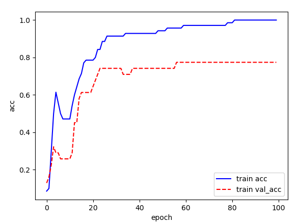
# 단어 단위 생성 모델 학습
from tensorflow.keras.preprocessing.sequence import pad_sequences

def testmodel(epoch, logs):
    if epoch % 5 != 0 and epoch != 49:
        return
    test_sentence = train_text[0]

    next_words = 100
    for _ in range(next_words):
        test_text_X = test_sentence.split(' ')[-seq_length:]
        test_text_X = np.array([word2idx[c] if c in word2idx else word2idx['UNK'] for c in test_text_X])
        test_text_X = pad_sequences([test_text_X], maxlen=seq_length, padding='pre', value=word2idx['UNK'])

        output_idx = model.predict_classes(test_text_X)
        test_sentence += ' ' + idx2word[output_idx[0]]
    
    print()
    print(test_sentence)
    print()

# 모델을 학습시키며 모델이 생성한 결과물을 확인하기 위해 LambdaCallback 함수 생성
testmodelcb = tf.keras.callbacks.LambdaCallback(on_epoch_end=testmodel)

history = model.fit(train_dataset.repeat(), epochs=50, 
                steps_per_epoch=steps_per_epoch, 
                callbacks=[testmodelcb], verbose=2)

model.save('rnnmodel.hdf5')
del model
from tensorflow.keras.models import load_model
model=load_model('rnnmodel.hdf5')

# 임의의 문장을 사용한 생성 결과 확인
test_sentence = '최참판댁 사랑은 무인지경처럼 적막하다'
#test_sentence = '동헌에 나가 공무를 본 후 활 십오 순을 쏘았다'

next_words = 500
for _ in range(next_words):
    # 임의 문장 입력 후 뒤에서 부터 seq_length 만킁ㅁ의 단어(25개) 선택
    test_text_X = test_sentence.split(' ')[-seq_length:]  
    
    # 문장의 단어를 인덱스 토큰으로 바꿈. 사전에 등록되지 않은 경우에는 'UNK' 코큰값으로 변경
    test_text_X = np.array([word2idx[c] if c in word2idx else word2idx['UNK'] for c in test_text_X])
    # 문장의 앞쪽에 빈자리가 있을 경우 25개 단어가 채워지도록 패딩
    test_text_X = pad_sequences([test_text_X], maxlen=seq_length, padding='pre', value=word2idx['UNK'])
    
    # 출력 중에서 가장 값이 큰 인덱스 반환
    output_idx = model.predict_classes(test_text_X) 
    test_sentence += ' ' + idx2word[output_idx[0]] # 출력단어는 test_sentence에 누적해 다음 스테의 입력으로 활용

print(test_sentence)


# LambdaCallback
# keras에서 여러가지 상황에서 콜백이되는 class들이 만들어져 있는데, LambdaCallback 등의 Callback class들은 
# 기본적으로 keras.callbacks.Callback class를 상속받아서 특정 상황마다 콜백되는 메소드들을 재정의하여 사용합니다. 
# LambdaCallback는 lambda 평션을 작성하여 생성자에 넘기는 방식으로 사용 할 수 있습니다. 
# callback 시 받는 arg는 Callbakc class에 정의 되어 있는대로 맞춰 주어야 합니다. 
# on_epoch_end메소드로 정의하여 epoch이 끝날 때 마다 확인해보도록 하겠습니다.
# 아래 처럼 lambda 함수를 작성하여 LambdaCallback를 만들어 주고, 이때 epoch, logs는 신경 안쓰시고 arg 형태만 맞춰주면 됩니다.
# from keras.callbacks import LambdaCallback
# print_weights = LambdaCallback(on_epoch_end=lambda epoch, logs: print(model.layers[3].get_weights()))

 - jamo tools

dschloe.github.io/python/tensorflow2.0/ch7_4_naturallanguagegeneration2/

 * tf_rnn9_토지_자소단위.ipynb

!pip install jamotools

import tensorflow as tf
import numpy as np
import jamotools

path_to_file = tf.keras.utils.get_file('toji.txt', 'https://raw.githubusercontent.com/pykwon/etc/master/rnn_test_toji.txt')
#path_to_file = 'silrok.txt'
# 데이터 로드 및 확인. encoding 형식으로 utf-8 을 지정해야합니다.
train_text = open(path_to_file, 'rb').read().decode(encoding='utf-8')

# 텍스트가 총 몇 자인지 확인합니다.
print('Length of text: {} characters'.format(len(train_text))) # Length of text: 695685 characters
print()

# 처음 100 자를 확인해봅니다.
s = train_text[:100]
print(s)

# 한글 텍스트를 자모 단위로 분리해줍니다. 한자 등에는 영향이 없습니다.
s_split = jamotools.split_syllables(s)
print(s_split)

Length of text: 695685 characters

제 1 편 어둠의 발소리
1897년의 한가위.
까치들이 울타리 안 감나무에 와서 아침 인사를 하기도 전에, 무색 옷에 댕기꼬리를 늘인 
아이들은 송편을 입에 물고 마을길을 쏘
ㅈㅔ 1 ㅍㅕㄴ ㅇㅓㄷㅜㅁㅇㅢ ㅂㅏㄹㅅㅗㄹㅣ
1897ㄴㅕㄴㅇㅢ ㅎㅏㄴㄱㅏㅇㅟ.
ㄲㅏㅊㅣㄷㅡㄹㅇㅣ ㅇㅜㄹㅌㅏㄹㅣ ㅇㅏㄴ ㄱㅏㅁㄴㅏㅁㅜㅇㅔ ㅇㅘㅅㅓ ㅇㅏㅊㅣㅁ ㅇㅣㄴㅅㅏㄹㅡㄹ ㅎㅏㄱㅣㄷㅗ ㅈㅓㄴㅇㅔ, ㅁㅜㅅㅐㄱ ㅇㅗㅅㅇㅔ ㄷㅐㅇㄱㅣㄲㅗㄹㅣㄹㅡㄹ ㄴㅡㄹㅇㅣㄴ 
ㅇㅏㅇㅣㄷㅡㄹㅇㅡㄴ ㅅㅗㅇㅍㅕㄴㅇㅡㄹ ㅇㅣㅂㅇㅔ ㅁㅜㄹㄱㅗ ㅁㅏㅇㅡㄹㄱㅣㄹㅇㅡㄹ ㅆㅗ

import jamotools

jamotools.split_syllables(s) : 

# 7.45 자모 결합 테스트
s2 = jamotools.join_jamos(s_split)
print(s2)
print(s == s2)

# 7.46 자모 토큰화
# 텍스트를 자모 단위로 나눕니다. 데이터가 크기 때문에 약간 시간이 걸립니다.
train_text_X = jamotools.split_syllables(train_text)
vocab = sorted(set(train_text_X))
vocab.append('UNK')
print ('{} unique characters'.format(len(vocab))) # 179 unique characters

# vocab list를 숫자로 맵핑하고, 반대도 실행합니다.
char2idx = {u:i for i, u in enumerate(vocab)}
idx2char = np.array(vocab)

text_as_int = np.array([char2idx[c] for c in train_text_X])
print(text_as_int) # [69 81  2 ...  2  1  0]

# word2idx 의 일부를 알아보기 쉽게 print 해봅니다.
print('{')
for char,_ in zip(char2idx, range(10)):
    print('  {:4s}: {:3d},'.format(repr(char), char2idx[char]))
print('  ...\n}')

print('index of UNK: {}'.format(char2idx['UNK']))

제 1 편 어둠의 발소리
1897년의 한가위.
까치들이 울타리 안 감나무에 와서 아침 인사를 하기도 전에, 무색 옷에 댕기꼬리를 늘인 
아이들은 송편을 입에 물고 마을길을 쏘
True
179 unique characters
[69 81  2 ...  2  1  0]
{
  '\n':   0,
  '\r':   1,
  ' ' :   2,
  '!' :   3,
  '"' :   4,
  "'" :   5,
  '(' :   6,
  ')' :   7,
  ',' :   8,
  '-' :   9,
  ...
}
index of UNK: 178

# 7.47 토큰 데이터 확인
print(train_text_X[:20])
print(text_as_int[:20])

# 7.48 학습 데이터세트 생성
seq_length = 80
examples_per_epoch = len(text_as_int) // seq_length
print('examples_per_epoch :', examples_per_epoch)
# examples_per_epoch : 16815
char_dataset = tf.data.Dataset.from_tensor_slices(text_as_int)

char_dataset = char_dataset.batch(seq_length+1, drop_remainder=True) # drop_remainder : 잔여 데이터 제거
for item in char_dataset.take(1):
    print(idx2char[item.numpy()])
#     ['ㅈ' 'ㅔ' ' ' '1' ' ' 'ㅍ' 'ㅕ' 'ㄴ' ' ' 'ㅇ' 'ㅓ' 'ㄷ' 'ㅜ' 'ㅁ' 'ㅇ' 'ㅢ' ' ' 'ㅂ'
#  'ㅏ' 'ㄹ' 'ㅅ' 'ㅗ' 'ㄹ' 'ㅣ' '\r' '\n' '1' '8' '9' '7' 'ㄴ' 'ㅕ' 'ㄴ' 'ㅇ' 'ㅢ' ' '
#  'ㅎ' 'ㅏ' 'ㄴ' 'ㄱ' 'ㅏ' 'ㅇ' 'ㅟ' '.' '\r' '\n' 'ㄲ' 'ㅏ' 'ㅊ' 'ㅣ' 'ㄷ' 'ㅡ' 'ㄹ' 'ㅇ'
#  'ㅣ' ' ' 'ㅇ' 'ㅜ' 'ㄹ' 'ㅌ' 'ㅏ' 'ㄹ' 'ㅣ' ' ' 'ㅇ' 'ㅏ' 'ㄴ' ' ' 'ㄱ' 'ㅏ' 'ㅁ' 'ㄴ'
#  'ㅏ' 'ㅁ' 'ㅜ' 'ㅇ' 'ㅔ' ' ' 'ㅇ' 'ㅘ' 'ㅅ']
    print('item.numpy() :', item.numpy())
# item.numpy() : [69 81  2 13  2 74 82 49  2 68 80 52 89 62 68 95  2 63 76 54 66 84 54 96
#   1  0 13 20 21 19 49 82 49 68 95  2 75 76 49 46 76 68 92 10  1  0 47 76
#  71 96 52 94 54 68 96  2 68 89 54 73 76 54 96  2 68 76 49  2 46 76 62 49
#  76 62 89 68 81  2 68 85 66]

def split_input_target(chunk):
    return [chunk[:-1], chunk[-1]]

train_dataset = char_dataset.map(split_input_target)
for x,y in train_dataset.take(1):
    print(idx2char[x.numpy()])
    print(x.numpy())
    print(idx2char[y.numpy()])
    print(y.numpy())
    
BATCH_SIZE = 64
steps_per_epoch = examples_per_epoch // BATCH_SIZE
BUFFER_SIZE = 5000

train_dataset = train_dataset.shuffle(BUFFER_SIZE).batch(BATCH_SIZE, drop_remainder=True)

ㅈㅔ 1 ㅍㅕㄴ ㅇㅓㄷㅜㅁㅇㅢ ㅂㅏㄹ
[69 81  2 13  2 74 82 49  2 68 80 52 89 62 68 95  2 63 76 54]
examples_per_epoch : 16815
['ㅈ' 'ㅔ' ' ' '1' ' ' 'ㅍ' 'ㅕ' 'ㄴ' ' ' 'ㅇ' 'ㅓ' 'ㄷ' 'ㅜ' 'ㅁ' 'ㅇ' 'ㅢ' ' ' 'ㅂ'
 'ㅏ' 'ㄹ' 'ㅅ' 'ㅗ' 'ㄹ' 'ㅣ' '\r' '\n' '1' '8' '9' '7' 'ㄴ' 'ㅕ' 'ㄴ' 'ㅇ' 'ㅢ' ' '
 'ㅎ' 'ㅏ' 'ㄴ' 'ㄱ' 'ㅏ' 'ㅇ' 'ㅟ' '.' '\r' '\n' 'ㄲ' 'ㅏ' 'ㅊ' 'ㅣ' 'ㄷ' 'ㅡ' 'ㄹ' 'ㅇ'
 'ㅣ' ' ' 'ㅇ' 'ㅜ' 'ㄹ' 'ㅌ' 'ㅏ' 'ㄹ' 'ㅣ' ' ' 'ㅇ' 'ㅏ' 'ㄴ' ' ' 'ㄱ' 'ㅏ' 'ㅁ' 'ㄴ'
 'ㅏ' 'ㅁ' 'ㅜ' 'ㅇ' 'ㅔ' ' ' 'ㅇ' 'ㅘ' 'ㅅ']
item.numpy() : [69 81  2 13  2 74 82 49  2 68 80 52 89 62 68 95  2 63 76 54 66 84 54 96
  1  0 13 20 21 19 49 82 49 68 95  2 75 76 49 46 76 68 92 10  1  0 47 76
 71 96 52 94 54 68 96  2 68 89 54 73 76 54 96  2 68 76 49  2 46 76 62 49
 76 62 89 68 81  2 68 85 66]
['ㅈ' 'ㅔ' ' ' '1' ' ' 'ㅍ' 'ㅕ' 'ㄴ' ' ' 'ㅇ' 'ㅓ' 'ㄷ' 'ㅜ' 'ㅁ' 'ㅇ' 'ㅢ' ' ' 'ㅂ'
 'ㅏ' 'ㄹ' 'ㅅ' 'ㅗ' 'ㄹ' 'ㅣ' '\r' '\n' '1' '8' '9' '7' 'ㄴ' 'ㅕ' 'ㄴ' 'ㅇ' 'ㅢ' ' '
 'ㅎ' 'ㅏ' 'ㄴ' 'ㄱ' 'ㅏ' 'ㅇ' 'ㅟ' '.' '\r' '\n' 'ㄲ' 'ㅏ' 'ㅊ' 'ㅣ' 'ㄷ' 'ㅡ' 'ㄹ' 'ㅇ'
 'ㅣ' ' ' 'ㅇ' 'ㅜ' 'ㄹ' 'ㅌ' 'ㅏ' 'ㄹ' 'ㅣ' ' ' 'ㅇ' 'ㅏ' 'ㄴ' ' ' 'ㄱ' 'ㅏ' 'ㅁ' 'ㄴ'
 'ㅏ' 'ㅁ' 'ㅜ' 'ㅇ' 'ㅔ' ' ' 'ㅇ' 'ㅘ']
[69 81  2 13  2 74 82 49  2 68 80 52 89 62 68 95  2 63 76 54 66 84 54 96
  1  0 13 20 21 19 49 82 49 68 95  2 75 76 49 46 76 68 92 10  1  0 47 76
 71 96 52 94 54 68 96  2 68 89 54 73 76 54 96  2 68 76 49  2 46 76 62 49
 76 62 89 68 81  2 68 85]
ㅅ
66

# 7.49 자소 단위 생성 모델 정의
total_chars = len(vocab)
model = tf.keras.Sequential([
    tf.keras.layers.Embedding(total_chars, 100, input_length=seq_length),
    tf.keras.layers.LSTM(units=400, activation='tanh'),
    tf.keras.layers.Dense(total_chars, activation='softmax')
])

model.compile(optimizer='adam', loss='sparse_categorical_crossentropy', metrics=['accuracy'])
model.summary()   # Total params: 891,279

# 7.50 자소 단위 생성 모델 학습
from tensorflow.keras.preprocessing.sequence import pad_sequences

def testmodel(epoch, logs):
    if epoch % 5 != 0 and epoch != 99:
        return
    
    test_sentence = train_text[:48]
    test_sentence = jamotools.split_syllables(test_sentence)

    next_chars = 300
    for _ in range(next_chars):
        test_text_X = test_sentence[-seq_length:]
        test_text_X = np.array([char2idx[c] if c in char2idx else char2idx['UNK'] for c in test_text_X])
        test_text_X = pad_sequences([test_text_X], maxlen=seq_length, padding='pre', value=char2idx['UNK'])

        output_idx = model.predict_classes(test_text_X)
        test_sentence += idx2char[output_idx[0]]
    
    print()
    print(jamotools.join_jamos(test_sentence))
    print()

testmodelcb = tf.keras.callbacks.LambdaCallback(on_epoch_end=testmodel)

history = model.fit(train_dataset.repeat(), epochs=50, steps_per_epoch=steps_per_epoch, \
                    callbacks=[testmodelcb], verbose=2)

Epoch 1/50
262/262 - 37s - loss: 2.9122 - accuracy: 0.2075
/usr/local/lib/python3.7/dist-packages/tensorflow/python/keras/engine/sequential.py:450: UserWarning: `model.predict_classes()` is deprecated and will be removed after 2021-01-01. Please use instead:* `np.argmax(model.predict(x), axis=-1)`,   if your model does multi-class classification   (e.g. if it uses a `softmax` last-layer activation).* `(model.predict(x) > 0.5).astype("int32")`,   if your model does binary classification   (e.g. if it uses a `sigmoid` last-layer activation).
  warnings.warn('`model.predict_classes()` is deprecated and '

제 1 편 어둠의 발소리
1897년의 한가위.
까치들이 울타리 안 감나무에 와서 안이이 알이이 알이이 알이이 알이이 알이이 알이이 알이이 알이이 알이이 알이이 알이이 알이이 알이이 알이이 알이이 알이이 알이이 알이이 알이이 알이이 알이이 알이이 알이이 알이이 알이이 알이이 알이이 알이이 알이이 알이이 알이이 알이이 알이이 알이이 알이이 알이이 알잉

Epoch 2/50
262/262 - 7s - loss: 2.3712 - accuracy: 0.3002
Epoch 3/50
262/262 - 7s - loss: 2.2434 - accuracy: 0.3256
Epoch 4/50
262/262 - 7s - loss: 2.1652 - accuracy: 0.3414
Epoch 5/50
262/262 - 7s - loss: 2.1132 - accuracy: 0.3491
Epoch 6/50
262/262 - 7s - loss: 2.0670 - accuracy: 0.3600

제 1 편 어둠의 발소리
1897년의 한가위.
까치들이 울타리 안 감나무에 와서 았다.  "아난 강이는 갈이는 갈이는 갈이는 갈이는 갈이는 갈이는 갈이는 갈이는 갈이는 갈이는 갈이는 갈이는 갈이는 갈이는 갈이는 갈이는 갈이는 갈이는 갈이는 갈이는 갈이는 갈이는 갈이는 갈이는 갈이는 갈이는 갈이는 갈이는 갈이는 갈이는 갈이는

Epoch 7/50
262/262 - 7s - loss: 2.0299 - accuracy: 0.3709
Epoch 8/50
262/262 - 7s - loss: 1.9852 - accuracy: 0.3810
Epoch 9/50
262/262 - 7s - loss: 1.9415 - accuracy: 0.3978
Epoch 10/50
262/262 - 7s - loss: 1.9119 - accuracy: 0.4020
Epoch 11/50
262/262 - 7s - loss: 1.8684 - accuracy: 0.4153

제 1 편 어둠의 발소리
1897년의 한가위.
까치들이 울타리 안 감나무에 와서 아니라고 날 간 간 간 간 간 간 간 간 간 간 간 간 간 간 간 간 간 간 간 간 간 간 간 간 간 간 간 간 간 간 간 간 간 간 간 간 간 간 간 간 간 간 간 간 간 간 간 간 간 간 간 간 간 간 간 간 간 간 간 간 간 간 간 간 간 간 간 간 간 간 간 간 ㄱ

Epoch 12/50
262/262 - 7s - loss: 1.8237 - accuracy: 0.4272
Epoch 13/50
262/262 - 7s - loss: 1.7745 - accuracy: 0.4429
Epoch 14/50
262/262 - 7s - loss: 1.7272 - accuracy: 0.4625
Epoch 15/50
262/262 - 7s - loss: 1.6779 - accuracy: 0.4688
Epoch 16/50
262/262 - 7s - loss: 1.6217 - accuracy: 0.4902

제 1 편 어둠의 발소리
1897년의 한가위.
까치들이 울타리 안 감나무에 와서 안 간 간 간 간 간 간 간 간 간 간 간 간 간 간 간 간 간 간 간 간 간 간 간 간 간 간 간 간 간 간 간 간 간 간 간 간 간 간 간 간 간 간 간 간 간 간 간 간 간 간 간 간 간 간 간 간 간 간 간 간 간 간 간 간 간 간 간 간 간 간 간 간 간 간 가

Epoch 17/50
262/262 - 7s - loss: 1.5658 - accuracy: 0.5041
Epoch 18/50
262/262 - 7s - loss: 1.4984 - accuracy: 0.5252
Epoch 19/50
262/262 - 7s - loss: 1.4413 - accuracy: 0.5443
Epoch 20/50
262/262 - 7s - loss: 1.3629 - accuracy: 0.5704
Epoch 21/50
262/262 - 7s - loss: 1.2936 - accuracy: 0.5923

제 1 편 어둠의 발소리
1897년의 한가위.
까치들이 울타리 안 감나무에 와서 아니요."
  "아는 말이 잡아낙에 사람 가나가 가라. 가나구가 가람 가나고. 사남이 바람이 그렇게 없는 노루가 가나가오. 아니라."
  "아는 말이 잡아낙에 사람 가나가 가라. 가나구가 가람 가나고. 사남이 바람이 그렇게 없는 노루가 가나가오. 아니라."
  "아는 말이 잡아낙에 사람 가나가 ㄱ

Epoch 22/50
262/262 - 7s - loss: 1.2142 - accuracy: 0.6217
Epoch 23/50
262/262 - 7s - loss: 1.1281 - accuracy: 0.6505
Epoch 24/50
262/262 - 7s - loss: 1.0444 - accuracy: 0.6786
Epoch 25/50
262/262 - 7s - loss: 0.9711 - accuracy: 0.7047
Epoch 26/50
262/262 - 7s - loss: 0.8712 - accuracy: 0.7445

제 1 편 어둠의 발소리
1897년의 한가위.
까치들이 울타리 안 감나무에 와서 아니요."
  "예, 서방이 타람 자기 있는 놀을 벤  앙이는  곡서방을 마지 않았다. 장모수는 잠 밀 앞은 알 앞은 것이다. 그러나 속으로 나랑치를  그렇더면 정을 비한 것은 알굴이 말고 마른 안 부리 전 물어지를 하는 것이다. 그런 소릴 긴데 없는  갈아조 말 앞은 ㅇ

Epoch 27/50
262/262 - 7s - loss: 0.8168 - accuracy: 0.7620
Epoch 28/50
262/262 - 7s - loss: 0.7244 - accuracy: 0.7985
Epoch 29/50
262/262 - 7s - loss: 0.6301 - accuracy: 0.8362
Epoch 30/50
262/262 - 7s - loss: 0.5399 - accuracy: 0.8695
Epoch 31/50
262/262 - 7s - loss: 0.4745 - accuracy: 0.8950

제 1 편 어둠의 발소리
1897년의 한가위.
까치들이 울타리 안 감나무에 와서 아니요."
 "그건 치신하게 소기일이고 나랑치가  가래 참아노려 하고 사람을 딸려들  하더나건서반다.
 "줄에 나무장 다과 있는데 마을 세나강이 사이오. 나익은 노영은 물을 딸로나 잉인이의 얼굴이  없고 바람을 들었다. 그 천덕이 속을 거밀렀다. 지녁해지직 때 났는데 이 ㅇ

Epoch 32/50
262/262 - 7s - loss: 0.3956 - accuracy: 0.9234
Epoch 33/50
262/262 - 7s - loss: 0.3326 - accuracy: 0.9429
Epoch 34/50
262/262 - 7s - loss: 0.2787 - accuracy: 0.9577
Epoch 35/50
262/262 - 7s - loss: 0.2249 - accuracy: 0.9738
Epoch 36/50
262/262 - 7s - loss: 0.1822 - accuracy: 0.9837

제 1 편 어둠의 발소리
1897년의 한가위.
까치들이 울타리 안 감나무에 와서 아니요."
 "그래 갱째기를 하였던 것이다. 그러나 소습으로  있을 물었다. 가나게, 한장한다. 
 "안 빌리 장에서  나였다. 체신기린 조한 시릴 세에 있이는 노랭이 되었다. 나무지 족은 야우는 물을 만다.  울씨는 지소 가라! 담하는 누눌이 말씨갔다. 
 "일서 좀은 이융이의 ㄴ

Epoch 37/50
262/262 - 7s - loss: 0.1399 - accuracy: 0.9902
Epoch 38/50
262/262 - 7s - loss: 0.1123 - accuracy: 0.9942
Epoch 39/50
262/262 - 7s - loss: 0.0864 - accuracy: 0.9968
Epoch 40/50
262/262 - 7s - loss: 0.0713 - accuracy: 0.9979
Epoch 41/50
262/262 - 7s - loss: 0.0552 - accuracy: 0.9989

제 1 편 어둠의 발소리
1897년의 한가위.
까치들이 울타리 안 감나무에 와서 아니요."
  "전을 짐 집 갚고 불랑이 떳어지는 닷마닥네서 쑤어직 때 가자. 다동이 타타자그마."
  "전을 지작한고, 그런 세닉을 바들 가는고 마진 오를 기는 불림이 최치른다. 한 일을 물었다.
  "눈저 살아노, 흔자하는 나루에."
  "저는 물을 물어져들  자몬 아니요."
  

Epoch 42/50
262/262 - 7s - loss: 0.0431 - accuracy: 0.9994
Epoch 43/50
262/262 - 7s - loss: 0.0325 - accuracy: 0.9998
Epoch 44/50
262/262 - 7s - loss: 0.2960 - accuracy: 0.9110
Epoch 45/50
262/262 - 7s - loss: 0.1939 - accuracy: 0.9540
Epoch 46/50
262/262 - 7s - loss: 0.0542 - accuracy: 0.9979

제 1 편 어둠의 발소리
1897년의 한가위.
까치들이 울타리 안 감나무에 와서 아니요."
  "전을 떰은 탕첫
은 안나무네."
  "그건 심심해 사람을 놀었다. 음....간 들지 휜 오를 
까끄치올을 쓸어얐다. 베여 갈인 덧못이야. 그건 시김이 잡아나게 생가가지가 다라고들 하고 사람들 색했으면 조신 소리를 필징이 갔다. 체공인 든장은 무소 그러핬다

Epoch 47/50
262/262 - 7s - loss: 0.0265 - accuracy: 0.9999
Epoch 48/50
262/262 - 7s - loss: 0.0189 - accuracy: 1.0000
Epoch 49/50
262/262 - 7s - loss: 0.0156 - accuracy: 1.0000
Epoch 50/50
262/262 - 7s - loss: 0.0131 - accuracy: 1.0000

model.save('rnnmodel2.hdf5')

# 7.51 임의의 문장을 사용한 생성 결과 확인
from tensorflow.keras.preprocessing.sequence import pad_sequences
test_sentence = '최참판댁 사랑은 무인지경처럼 적막하다'
test_sentence = jamotools.split_syllables(test_sentence)

next_chars = 5000
for _ in range(next_chars):
    test_text_X = test_sentence[-seq_length:]
    test_text_X = np.array([char2idx[c] if c in char2idx else char2idx['UNK'] for c in test_text_X])
    test_text_X = pad_sequences([test_text_X], maxlen=seq_length, padding='pre', value=char2idx['UNK'])
    
    output_idx = model.predict_classes(test_text_X)
    test_sentence += idx2char[output_idx[0]]
    

print(jamotools.join_jamos(test_sentence))

/usr/local/lib/python3.7/dist-packages/tensorflow/python/keras/engine/sequential.py:450: UserWarning: `model.predict_classes()` is deprecated and will be removed after 2021-01-01. Please use instead:* `np.argmax(model.predict(x), axis=-1)`,   if your model does multi-class classification   (e.g. if it uses a `softmax` last-layer activation).* `(model.predict(x) > 0.5).astype("int32")`,   if your model does binary classification   (e.g. if it uses a `sigmoid` last-layer activation).
  warnings.warn('`model.predict_classes()` is deprecated and '
최참판댁 사랑은 무인지경처럼 적막하다가 최차는 야우는 물을 물었다.
  "내가 적에서 이자사 아니요."
  "전을 떰은 안 불이라 강천 갓촉을 농해 났이 마으러서 같은 노웅이 것을  치문이 참만난 함잉이의 송순이라 강을 덜걱을  눈치를  최철었다.
  "오를 놀짝은 노영은 뭇
이들을 달려들  도만 살알이 되었다. 나무지 족은 야움을 놀을 허렸다. 그건 신기를 물을 달려들 딸을 동렸다. 
“선으로 바람 사람을 바습으로 나왔다. 
간가나게, 사람들 사람을  했는 노래원이 머를 세 있는 것 같았다.
  강산이 족은 양피는 가날이 아니요."
  "예, 산고 가탕이 다시 죽얼 지 구천하게  그러세 얼굴을 달련 덧을  부칠리 질 없는 농은 언분네요."
  "그건 소리가 아니물이 용닌이 되수  성을 흠금글고 달려가지 아나갔다. 
 "그러나 내간이고 내발이 탂어서 달려가지 않나. 무고 고랭각은 다사 죽어러들어지 않았다. 
간곡이얐다. 지낙해지 안 가기요."
 "잔은 안 불린 것 같았다.
  강산이 종굴이  왔고 싶은 상모수는 곳한 곰집은 것 같았다.
  강산이 족은 양피는 가날이 아니요."
  "예, 산고 가탕이 다시 죽얼 지 구천하게  그러세 얼굴을 달련 덧을  부칠리 질 없는 농은 언분네요."
  "그건 소리가 아니물이 용닌이 되수  성을 흠금글고 달려가지 아나갔다. 
 "그러나 내간이고 내발이 탂어서 달려가지 않나. 무고 고랭각은 다사 죽어러들어지 않았다. 
간곡이얐다. 지낙해지 안 가기요."
 "잔은 안 불린 것 같았다.
  강산이 종굴이  왔고 싶은 상모수는 곳한 곰집은 것 같았다.
  강산이 족은 양피는 가날이 아니요."
  "예, 산고 가탕이 다시 죽얼 지 구천하게  그러세 얼굴을 달련 덧을  부칠리 질 없는 농은 언분네요."
  "그건 소리가 아니물이 용닌이 되수  성을 흠금글고 달려가지 아나갔다. 
 "그러나 내간이고 내발이 탂어서 달려가지 않나. 무고 고랭각은 다사 죽어러들어지 않았다. 
간곡이얐다. 지낙해지 안 가기요."
 "잔은 안 불린 것 같았다.
  강산이 종굴이  왔고 싶은 상모수는 곳한 곰집은 것 같았다.
  강산이 족은 양피는 가날이 아니요."
  "예, 산고 가탕이 다시 죽얼 지 구천하게  그러세 얼굴을 달련 덧을  부칠리 질 없는 농은 언분네요."
  "그건 소리가 아니물이 용닌이 되수  성을 흠금글고 달려가지 아나갔다. 
 "그러나 내간이고 내발이 탂어서 달려가지 않나. 무고 고랭각은 다사 죽어러들어지 않았다. 
간곡이얐다. 지낙해지 안 가기요."
 "잔은 안 불린 것 같았다.
  강산이 종굴이  왔고 싶은 상모수는 곳한 곰집은 것 같았다.
  강산이 족은 양피는 가날이 아니요."
  "예, 산고 가탕이 다시 죽얼 지 구천하게  그러세 얼굴을 달련 덧을  부칠리 질 없는 농은 언분네요."
  "그건 소리가 아니물이 용닌이 되수  성을 흠금글고 달려가지 아나갔다. 
 "그러나 내간이고 내발이 탂어서 달려가지 않나. 무고 고랭각은 다사 죽어러들어지 않았다. 
간곡이얐다. 지낙해지 안 가기요."
 "잔은 안 불린 것 같았다.
  강산이 종굴이  왔고 싶은 상모수는 곳한 곰집은 것 같았다.
  강산이 족은 양피는 가날이 아니요."
  "예, 산고 가탕이 다시 죽얼 지 구천하게  그러세 얼굴을 달련 덧을  부칠리 질 없는 농은 언분네요."
  "그건 소리가 아니물이 용닌이 되수  성을 흠금글고 달려가지 아나갔다. 
 "그러나 내간이고 내발이 탂어서 달려가지 않나. 무고 고랭각은 다사 죽어러들어지 않았다. 
간곡이얐다. 지낙해지 안 가기요."
 "잔은 안 불린 것 같았다.
  강산이 종굴이  왔고 싶은 상모수는 곳한 곰집은 것 같았다.
  강산이 족은 양피는 가날이 아니요."
  "예, 산고 가탕이 다시 죽얼 지 구천하게  그러세 얼굴을 달련 덧을  부칠리 질 없는 농은 언분네요."
  "그건 소리가 아니물이 용닌이 되수  성을 흠금글고 달려가지 아나갔다. 
 "그러나 내간이고 내발이 탂어서 달려가지 않나. 무고 고랭각은 다사 죽어러들어지 않았다. 
간곡이얐다. 지낙해지 안 가기요."
 "잔은 안 불린 것 같았다.
  강산이 종굴이  왔고 싶은 상모수는 곳한 곰집은 것 같았다.
  강산이 족은 양피는 가날이 아니요."
  "예, 산고 가탕이 다시 죽얼 지 구천하게  그러세 얼굴을 달련 덧을  부칠리 질 없는 농은 언분네요."
  "그건 소리가 아니물이 용닌이 되수  성을 흠금글고 달려가지 아나갔다. 
 "그러나 내간이고 내발이 탂어서 달려가지 않나. 무고 고랭각은 다사 죽어러들어지 않았다. 
간곡이얐다. 지낙해지 안 가기요."
 "잔은 안 불린 것 같았다.
  강산이 종굴이  왔고 싶은 상모수는 곳한 곰집은 것 같았다.
  강산이 족은 양피는 가날이 아니요."
  "예, 산고 가탕이 다시 죽얼 지 구천하게  그러세 얼굴을 달련 덧을  부칠리 질 없는 농은 언분네요."
  "그건 소리가 아니물이 용닌이 되수  성을 흠금글고 달려가지 아나갔다. 
 "그러나 내간이고 내발이 탂어서 달려가지 않나. 무고 고랭각은 다사 죽어러들어지 않았다. 
간곡이얐다. 지낙해지 안 가기요."
 "잔은 안 불린 것 같았다.
  강산이 종굴이  왔고 싶은 상모수는 곳한 곰지

RNN을 이용한 스펨메일 분류(이진 분류)

 * tf_rnn10_스팸메일분류.ipynb

import pandas as pd

data = pd.read_csv('https://raw.githubusercontent.com/pykwon/python/master/testdata_utf8/spam.csv', encoding='latin1')
print(data.head())
print('샘플 수 : ', len(data))                       # 샘플 수 :  5572
del data['Unnamed: 2']
del data['Unnamed: 3']
del data['Unnamed: 4']
print(data.head())
#      v1  ... Unnamed: 4
# 0   ham  ...        NaN
# 1   ham  ...        NaN
# 2  spam  ...        NaN
# 3   ham  ...        NaN
# 4   ham  ...        NaN
print(data.v1.unique())                              # ['ham' 'spam']
data['v1'] = data['v1'].replace(['ham', 'spam'], [0, 1])
print(data.head())

# Null 여부 확인
print(data.isnull().values.any())                     # False
print(data.info())

# 중복 데이터 확인
print(data['v2'].nunique())                           # 5169

data.drop_duplicates(subset=['v2'], inplace=True)
print('중복 데이터 제거 후 샘플 수 : ', len(data))    # 5169

print(data.groupby('v1').size().reset_index(name='count'))
#    v1  count
# 0   0   4516
# 1   1    653

# feature(v2), label(v1) 분리
xdata = data['v2']
ydata = data['v1']
print(xdata[:3])
# 0    Go until jurong point, crazy.. Available only ...
# 1                        Ok lar... Joking wif u oni...
# 2    Free entry in 2 a wkly comp to win FA Cup fina...

print(ydata[:3])
# 0    0
# 1    0
# 2    1

 - token 처리

from tensorflow.keras.preprocessing.text import Tokenizer
tok = Tokenizer()
tok.fit_on_texts(xdata)
print(tok.word_index) # {'i': 1, 'to': 2, 'you': 3, 'a': 4, 'the': 5, 'u': 6, 'and': 7, 'in': 8, 'is': 9, 'me': 10 ...
sequences = tok.texts_to_sequences(xdata)
print(xdata[:5])
# 0    Go until jurong point, crazy.. Available only ...
# 1                        Ok lar... Joking wif u oni...
# 2    Free entry in 2 a wkly comp to win FA Cup fina...
# 3    U dun say so early hor... U c already then say...
# 4    Nah I don't think he goes to usf, he lives aro...
print(sequences[:5])
# [[47, 433, 4013, 780, 705, 662, 64, 8, 1202, 94, 121, 434, 1203, ...
word_index = tok.word_index
print(word_index)
# {'i': 1, 'to': 2, 'you': 3, 'a': 4, 'the': 5, 'u': 6, 'and': 7, 'in': 8, 'is': 9, 'me': 10, ...
print(len(word_index)) # 8920

# 전체 자료 중 등장빈도 수, 비율 확인
threshold = 2                   # 등장빈도 수를 제한
total_count = len(word_index)   # 전체 단어 수
rare_count = 0                  # 빈도 수가 threshold 보다 작은 경우
total_freq = 0                  # 전체 단어 빈도 수 총합 비율
rare_freq = 0                   # 빈도 수 가 threshold보다 작은 경우의 단어 빈도 수 총합 비율 전체 자료 중 등장빈도 수, 비율 확인
threshold = 2                   # 등장빈도 수를 제한
total_count = len(word_index)   # 전체 단어 수
rare_count = 0                  # 빈도 수가 threshold 보다 작은 경우
total_freq = 0                  # 전체 단어 빈도 수 총합 비율
rare_freq = 0                   # 빈도 수 가 threshold보다 작은 경우의 단어 빈도 수 총합 비율

# dict type의 단어/빈도수 얻기
for key, value in tok.word_counts.items():
    #print('k:{} va:{}'.format(key, value))
    # k:jd va:1
    # k:accounts va:1
    # k:executive va:2
    # k:parents' va:2
    # k:picked va:7
    # k:downstem va:1
    # k:08718730555 va:
    total_freq = total_freq + value

    if value < threshold:
        rare_count = rare_count + 1
        rare_freq = rare_freq + value

print('등장빈도가 1회인 단어 수 :', rare_count)                                # 등장빈도가 1회인 단어 수 : 4908
print('등장빈도가 1회인 단어 비율 :', (rare_count / total_count) * 100)        # 등장빈도가 1회인 단어 비율 : 55.02242152466368
print('전체 중 등장빈도가 1회인 단어 비율 :', (rare_freq / total_freq) * 100)  # 전체 중 등장빈도가 1회인 단어 비율 : 6.082538108811501

tok = Tokenizer(num_words= total_count - rare_count + 1)

vocab_size = len(word_index) + 1
print('단어 집합 크기 :', vocab_size)   # 단어 집합 크기 : 8921

# train/test 8:2
n_of_train = int(len(sequences) * 0.8)
n_of_test = int(len(sequences) - n_of_train)
print('train lenghth :', n_of_train)    # train lenghth : 4135
print('test lenghth :', n_of_test)      # test lenghth : 1034

# 메일의 길이 확인
x_data = sequences
print('메일의 최대 길이 :', max((len(i) for i in x_data)))          # 메일의 최대 길이 : 189
print('메일의 평균 길이 :', (sum(map(len, x_data)) / len(x_data)))  # 메일의 평균 길이 : 15.610369510543626

# 시각화
import matplotlib.pyplot as plt
plt.hist([len(siz) for siz in x_data], bins=50)
plt.xlabel('length')
plt.ylabel('count')
plt.show()

from tensorflow.keras.preprocessing.sequence import pad_sequences
max_len = max((len(i) for i in x_data))
data = pad_sequences(x_data, maxlen=max_len)
print(data.shape)       # (5169, 189)

# train/test 분리
import numpy as np
x_train = data[:n_of_train]
y_train = np.array(ydata[:n_of_train])
x_test = data[n_of_train:]
y_test = np.array(ydata[n_of_train:])
print(x_train.shape, x_train[:2])   # (4135, 189)
print(y_train.shape, y_train[:2])   # (4135,)
print(x_test.shape, y_test.shape)   # (1034, 189) (1034,)

# 모델
from tensorflow.keras.layers import LSTM, Embedding, Dense, Dropout
from tensorflow.keras.models import Sequential

model = Sequential()
model.add(Embedding(vocab_size, 32))
model.add(LSTM(32, activation='tanh'))
model.add(Dense(32, activation='relu'))
model.add(Dropout(0.2))
model.add(Dense(1, activation='sigmoid'))
print(model.summary())      # Total params: 294,881

model.compile(optimizer='adam', loss='binary_crossentropy', metrics=['acc'])
history = model.fit(x_train, y_train, epochs=5, batch_size=32, validation_split=0.25, verbose=2)
print('loss, acc :', model.evaluate(x_test, y_test))    # loss, acc : [0.05419406294822693, 0.9893617033958435]

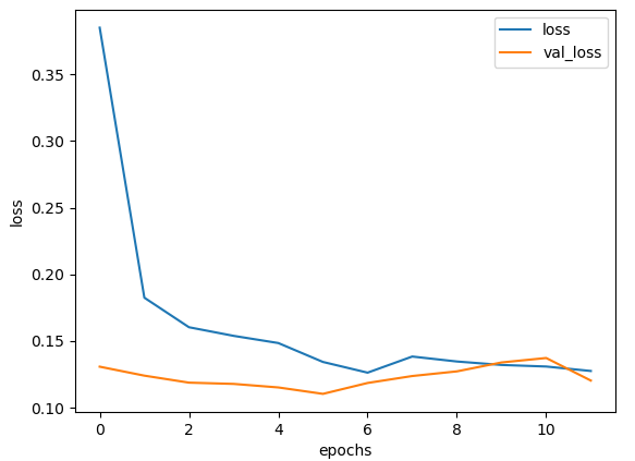
# print(x_test[0])

# loss, acc 변화에 대한 시각화
epochs = range(1, len(history.history['acc']) + 1)
plt.plot(epochs, history.history['loss'])
plt.plot(epochs, history.history['val_loss'])
plt.xlabel('epoch')
plt.ylabel('loss')
plt.legend(['train loss', 'validation_loss'])
plt.show()

plt.plot(epochs, history.history['acc'])
plt.plot(epochs, history.history['val_acc'])
plt.xlabel('epoch')
plt.ylabel('acc')
plt.legend(['train acc', 'validation_acc'])
plt.show()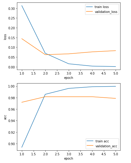

로이터 뉴스 분류하기

wikidocs.net/22933

Keras를 이용한 One-hot encoding, Embedding

cafe.daum.net/flowlife/S2Ul/19

dacon.io/codeshare/1892

wikidocs.net/33520

word2vec tf idf

blog.naver.com/PostView.nhn?blogId=happyrachy&logNo=221285427229&parentCategoryNo=&categoryNo=16&viewDate=&isShowPopularPosts=false&from=postView

 * tf_rnn11_뉴스카테고리분류.ipynb

import numpy as np
import tensorflow as tf
from tensorflow.keras.datasets import reuters
from tensorflow.keras.models import Sequential
from tensorflow.keras.layers import LSTM, Dense, Embedding
from tensorflow.keras.preprocessing import sequence
from tensorflow.keras.utils import to_categorical

np.random.seed(3)
tf.random.set_seed(3)

#print(reuters.load_data())
# (x_train, y_train), (x_test, y_test) = reuters.load_data()
# print(x_train.shape, y_train.shape, x_test.shape, y_test.shape) # (8982,) (8982,) (2246,) (2246,)

(x_train, y_train), (x_test, y_test) = reuters.load_data(num_words=1000, test_split=0.2) # test_split=0.2 default, num_words=1000 : 빈도 순위 1000이하 값만 출력
#(x_train, y_train), (x_test, y_test) = reuters.load_data(num_words=None, test_split=0.2) # test_split=0.2 default
print(x_train.shape, y_train.shape, x_test.shape, y_test.shape) # (8982,) (8982,) (2246,) (2246,)

category = np.max(y_train) + 1
print('category :', category)   # category : 46
print(x_train[:3])              # 숫자가 작을 수록 빈도수가 높음
# [list([1, 2, 2, 8, 43, 10, 447, 5, 25, 207, 270, 5, 2, 111, 16, 369, 186, 90, 67, 7, 89, ... 109, 15, 17, 12])
#  list([1, 2, 699, 2, 2, 56, 2, 2, 9, 56, 2, 2, 81, 5, 2, 57, 366, 737, 132, 20, 2, 7, 2, ...  2, 505, 17, 12])
#  list([1, 53, 12, 284, 15, 14, 272, 26, 53, 959, 32, 818, 15, 14, 272, 26, 39, 684, 70, ... 59, 11, 17, 12])]
print(y_train[:3])              # [3 4 3]
print(len(s) for s in x_train)

import matplotlib.pyplot as plt
plt.hist([len(s) for s in x_train], bins = 50)
plt.xlabel('length')
plt.ylabel('number')
plt.show()

 - 데이터 구성

word_index = reuters.get_word_index()
print(word_index)       # {'mdbl': 10996, 'fawc': 16260, 'degussa': 12089, 'woods': 8803, 'hanging': 13796, ... }

index_to_word = {}
for k, v in word_index.items():
    index_to_word[v] = k

print(index_to_word)    # {10996: 'mdbl', 16260: 'fawc', 12089: 'degussa', 8803: 'woods', 13796: 'hanging ... }
print(index_to_word[1]) # the
print(index_to_word[10])    # for
print(index_to_word[100])   # group

print(x_train[0])                                       # [1, 2, 2, 8, 43, 10, 447, 5, 25, 207, 270, 5, 2, 111, 16, 369, ...
print(' '.join(index_to_word[i] for i in x_train[0]))   # he of of mln loss for plc said at only ended said of  ... 

 - 모델

x_train = sequence.pad_sequences(x_train, maxlen=100)
x_test = sequence.pad_sequences(x_test, maxlen=100)
y_train = to_categorical(y_train)
y_test = to_categorical(y_test)
print(x_test)
# [[  0   0   0 ...  15  17  12]
#  [  0   0   0 ... 505  17  12]
#  [ 19 758  15 ...  11  17  12]
#  ...
#  [  0   0   0 ... 407  17  12]
#  [ 88   2  72 ... 364  17  12]
#  [125   2  21 ... 113  17  12]]
#print(y_test)

model = Sequential()
model.add(Embedding(1000, 100))
model.add(LSTM(100, activation='tanh'))
model.add(Dense(46, activation='softmax'))
print(model.summary())  # Total params: 185,046

model.compile(optimizer='adam', loss='categorical_crossentropy', metrics=['accuracy'])

history = model.fit(x_train, y_train, batch_size=64, epochs=50, validation_data=(x_test, y_test), verbose=2)

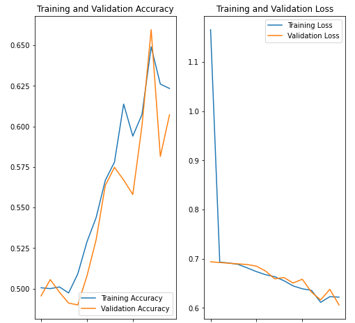
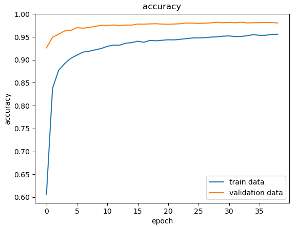
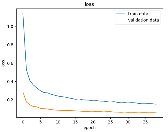
 - 시각화

vloss = history.history['val_loss']
loss = history.history['loss']
x_len = np.arange(len(loss))
plt.plot(x_len, vloss, marker='.', c='red', label='train val_loss')
plt.plot(x_len, loss, marker='o', c='blue', label='train loss')
plt.xlabel('epoch')
plt.ylabel('loss')
plt.legend()
plt.show()

vacc = history.history['val_accuracy']
acc = history.history['accuracy']
x_len = np.arange(len(acc))
plt.plot(x_len, vacc, marker='.', c='red', label='train val_acc')
plt.plot(x_len, acc, marker='o', c='blue', label='train acc')
plt.xlabel('epoch')
plt.ylabel('acc')
plt.legend()
plt.show()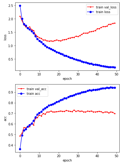

 - IMDB

wikidocs.net/24586

tf 2 에서 RNN(LSTM) sample

cafe.daum.net/flowlife/S2Ul/21

 * tf_rnn12_IMDB감성분류.ipynb

import numpy as np
import tensorflow as tf
from tensorflow.keras.datasets import imdb
from tensorflow.keras.models import Sequential
from tensorflow.keras.layers import LSTM, Dense, Embedding
from tensorflow.keras.preprocessing import sequence
from tensorflow.keras.utils import to_categorical
import matplotlib.pyplot as plt

np.random.seed(3)
tf.random.set_seed(3)
# print(imdb.load_data())
vocab_size = 10000
(x_train, y_train), (x_test, y_test) = imdb.load_data(num_words=vocab_size)
print(x_train.shape, y_train.shape, x_test.shape, y_test.shape) # (25000,) (25000,) (25000,) (25000,)

print(y_train[:3])                              # [1 0 0]
num_classes = max(y_train) + 1
print('num_classes :',num_classes)              # num_classes : 2
print(set(y_train), ' ', np.unique(y_train))    # {0, 1}   [0 1]

print(x_train[0])                               # [1, 14, 22, 16, 43, 530, 973, 1622, 1385, 65, 458, 4468, 66, 3941, ...
print(y_train[0])                               # 1

 - 시각화 : 훈련용 리뷰 분포

len_result = [len(s) for s in x_train]
print('리뷰 최대 길이 :', np.max(len_result))  # 2494
print('리뷰 평균 길이 :', np.mean(len_result)) # 238.71364

plt.subplot(1, 2, 1)
plt.boxplot(len_result)
plt.subplot(1, 2, 2)
plt.hist(len_result, bins=50)
plt.show()

 - 긍/부정 빈도수

unique_ele, counts_ele = np.unique(y_train, return_counts=True)
print(np.asarray((unique_ele, counts_ele)))
# [[    0     1]
#  [12500 12500]]

 - index에 대한 단어 출력

word_to_index = imdb.get_word_index()
index_to_word = {}
for k, v in word_to_index.items():
    index_to_word[v] = k
print(index_to_word)        # {34701: 'fawn', 52006: 'tsukino', 52007: 'nunnery', 16816: 'sonja', ...
print(index_to_word[1])     # the
print(index_to_word[1408])  # woods

print(x_train[0])           # [1, 14, 22, 16, 43, 530, 973, 1622, ...
print(y_train[0])           # 1
print(' '.join([index_to_word[index] for index in x_train[0]]))     # the as you with out themselves powerful lets loves their ...

 - LSTM으로 감성분류

from tensorflow.keras.preprocessing.sequence import pad_sequences
from tensorflow.keras.callbacks import EarlyStopping, ModelCheckpoint
from tensorflow.keras.models import load_model

max_len = 500
x_train = pad_sequences(x_train, maxlen=max_len)
x_test = pad_sequences(x_test, maxlen=max_len)
# print(x_train[0])

model = Sequential()
model.add(Embedding(vocab_size, 100))
model.add(LSTM(120, activation='tanh'))
model.add(Dense(1, activation='sigmoid'))

print(model.summary())      # Total params: 1,106,201

model.compile(loss='binary_crossentropy', optimizer='adam', metrics=['acc'])
es = EarlyStopping(monitor='val_loss', mode='auto', patience=3, baseline=0.01)
ms = ModelCheckpoint('tfrmm12.h5', monitor='val_acc', mode='max', save_best_only = True)
model.fit(x_train, y_train, validation_data=(x_test, y_test), epochs=100, batch_size=64, verbose=2, callbacks=[es, ms])

loaded_model = load_model('tfrmm12.h5')
print('acc :',loaded_model.evaluate(x_test, y_test)[1])     # acc : 0.8718400001525879
print('loss :',loaded_model.evaluate(x_test, y_test)[0])    # loss : 0.3080214262008667

 - CNN으로 텍스트 분류

from tensorflow.keras.layers import Conv1D, GlobalMaxPooling1D, MaxPooling1D, Dropout

model = Sequential()
model.add(Embedding(vocab_size, 256))
model.add(Conv1D(256, kernel_size=3, padding='valid', activation='relu', strides=1))
model.add(GlobalMaxPooling1D())
model.add(Dense(1, activation='sigmoid'))
print(model.summary())          # Total params: 2,757,121

model.compile(loss='binary_crossentropy', optimizer='adam', metrics=['acc'])
es = EarlyStopping(monitor='val_loss', mode='auto', patience=3, baseline=0.01)
ms = ModelCheckpoint('tfrmm12_1.h5', monitor='val_acc', mode='max', save_best_only = True)
history = model.fit(x_train, y_train, validation_data=(x_test, y_test), epochs=100, batch_size=64, verbose=2, callbacks=[es, ms])

loaded_model = load_model('tfrmm12_1.h5')
print('acc :',loaded_model.evaluate(x_test, y_test)[1])     # acc : 0.8984400033950806
print('loss :',loaded_model.evaluate(x_test, y_test)[0])    # loss : 0.24771703779697418

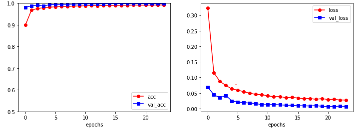
 - 시각화

vloss = history.history['val_loss']
loss = history.history['loss']
x_len = np.arange(len(loss))
plt.plot(x_len, vloss, marker='+', c='black', label='val_loss')
plt.plot(x_len, loss, marker='s', c='red', label='loss')
plt.legend()
plt.grid()
plt.show()

import re
def sentiment_predict(new_sentence):
  new_sentence = re.sub('[^0-9a-zA-Z ]', '', new_sentence).lower()

  # 정수 인코딩
  encoded = []
  for word in new_sentence.split():
    # 단어 집합의 크기를 10,000으로 제한.
    try :
      if word_to_index[word] <= 10000:
        encoded.append(word_to_index[word]+3)
      else:
        encoded.append(2)   # 10,000 이상의 숫자는 <unk> 토큰으로 취급.
    except KeyError:
      encoded.append(2)   # 단어 집합에 없는 단어는 <unk> 토큰으로 취급.

  pad_new = pad_sequences([encoded], maxlen = max_len) # 패딩
  
  # 예측하기
  score = float(loaded_model.predict(pad_new)) 
  if(score > 0.5):
    print("{:.2f}% 확률로 긍정!.".format(score * 100))
  else:
    print("{:.2f}% 확률로 부정!".format((1 - score) * 100))
# 99.57% 확률로 긍정!.
# 53.55% 확률로 긍정!.

# 긍/부정 분류 예측
#temp_str = "This movie was just way too overrated. The fighting was not professional and in slow motion."
temp_str = "This movie was a very touching movie."
sentiment_predict(temp_str)

temp_str = " I was lucky enough to be included in the group to see the advanced screening in Melbourne on the 15th of April, 2012. And, firstly, I need to say a big thank-you to Disney and Marvel Studios."
sentiment_predict(temp_str)

네이버 영화 리뷰 데이터를 이용해 분류 모델 작성

한국어 불용어, 토크나이징 툴

cafe.daum.net/flowlife/9A8Q/156

 * tf_rnn13_naver감성분류.ipynb

#! pip install konlpy

import numpy as np
import pandas as pd
import matplotlib as plt
import re
from konlpy.tag import Okt
from tensorflow.keras.layers import Embedding, Dense, LSTM, Dropout
from tensorflow.keras.models import Sequential, load_model
from tensorflow.keras.callbacks import EarlyStopping, ModelCheckpoint
from tensorflow.keras.preprocessing.text import Tokenizer
from tensorflow.keras.preprocessing.sequence import pad_sequences

train_data = pd.read_table('https://raw.githubusercontent.com/pykwon/python/master/testdata_utf8/ratings_train.txt')
test_data = pd.read_table('https://raw.githubusercontent.com/pykwon/python/master/testdata_utf8/ratings_test.txt')
print(train_data[:3], len(train_data))  # 150000
print(test_data[:3], len(test_data))    # 50000
#          id                           document  label
# 0   9976970                아 더빙.. 진짜 짜증나네요 목소리      0
# 1   3819312  흠...포스터보고 초딩영화줄....오버연기조차 가볍지 않구나      1
# 2  10265843                  너무재밓었다그래서보는것을추천한다      0
print(train_data.columns)               # Index(['id', 'document', 'label'], dtype='object')
# imsi = train_data.sample(n=1000, random_state=123)
# print(imsi)

 - 데이터 전처리

# 데이터 전처리
print(train_data['document'].nunique(), test_data['document'].nunique())    # 146182 49157 => 중복자료가 있다.

train_data.drop_duplicates(subset=['document'], inplace=True)               # 중복 제거
print(len(train_data['document']))  # 146183
print(set(train_data['label']))     # {0 부정, 1 긍정}

train_data['label'].value_counts().plot(kind='bar')
plt.show()

print(train_data.groupby('label').size())
# label
# 0    73342
# 1    72841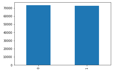

 - Null 값 확인

print(train_data.isnull().values.any()) # True
print(train_data.isnull().sum())
# id          0
# document    1
# label       0
print(train_data.loc[train_data.document.isnull()])
#             id document  label
# 25857  2172111      NaN      1

train_data = train_data.dropna(how='any')
print(train_data.isnull().values.any())     # False
print(len(train_data))                      # 146182

 - 순수 한글 관련 자료 이외의 구둣점 등은 제거

print(train_data[:3])
train_data['document'] = train_data['document'].str.replace("[^ㄱ-ㅎ ㅏ-ㅣ 가-힣]","")
print(train_data[:3])

train_data['document'].replace('', np.nan, inplace=True)
print(train_data.isnull().sum())
# id            0
# document    391
# label         0

train_data = train_data.dropna(how='any')
print(train_data.isnull().values.any()) # False
print(len(train_data))                  # 145791

# test
test_data.drop_duplicates(subset=['document'], inplace=True)               # 중복 제거
test_data['document'] = test_data['document'].str.replace("[^ㄱ-ㅎ ㅏ-ㅣ 가-힣]","")
test_data['document'].replace('', np.nan, inplace=True)
test_data = test_data.dropna(how='any')
print(test_data.isnull().values.any())  # False
print(len(test_data))                   # 48995

 - 불용어 제거 & 형태소 분류

# 불용어 제거
stopwords = ['아','휴','아이구','아이쿠','아이고','어','나','우리','저희','따라','의해','을','를','에','의','가','으로','로','에게','뿐이다','의거하여']

# 형태소 분류
okt = Okt()
x_train = []
for sen in train_data['document']:
    imsi = []
    imsi = okt.morphs(sen, stem=True)   # stem=True : 어간 추출
    imsi = [word for word in imsi if not word in stopwords]
    x_train.append(imsi)

print(x_train[:3])
# [['더빙', '진짜', '짜증나다', '목소리'], ['흠', '포스터', '보고', '초딩', '영화', '줄', '오버', '연기', '조차', '가볍다', '않다'], ['너', '무재', '밓었', '다그', '래서', '보다', '추천', '한', '다']]

x_test = []
for sen in test_data['document']:
    imsi = []
    imsi = okt.morphs(sen, stem=True)   # stem=True : 어간 추출
    imsi = [word for word in imsi if not word in stopwords]
    x_test.append(imsi)

print(x_test[:3])
# [['굳다', 'ㅋ'], ['뭐', '야', '이', '평점', '들', '은', '나쁘다', '않다', '점', '짜다', '리', '는', '더', '더욱', '아니다'], ['지루하다', '않다', '완전', '막장', '임', '돈', '주다', '보기', '에는']]

 - 워드 임베딩

tok = Tokenizer()
tok.fit_on_texts(x_train)
print(tok.word_index)
# {'이': 1, '영화': 2, '보다': 3, '하다': 4, '도': 5, '들': 6, '는': 7, '은': 8, '없다': 9, '이다': 10, '있다': 11, '좋다': 12, ...

 - 등장 빈도수를 확인해서 비중이 적은 자료는 배제

threshold = 3
total_cnt = len(tok.word_index)
rare_cnt = 0
total_freq = 0
rare_freq = 0

for k, v in tok.word_counts.items():
    total_freq = total_freq + v
    if v < threshold:
        rare_cnt = rare_cnt + 1
        rare_freq = rare_freq + v

print('total_cnt :', total_cnt)                         # 43753
print('rare_cnt :', rare_cnt)                           # 24340
print('rare_freq :', (rare_cnt / total_cnt) * 100)      # 55.63047105341348
print('total_cnt :', (rare_freq / total_freq) * 100)    # 1.71278110414947
# 2회 이하인 단어 전체 비중 1.7%이므로 2회 이하인 단어들은 배제해도 문제가 없을 것 같다

 - OOV(Out of Vocabulary) : 단어 사전에 없으면 index자체를 할 수 없게 되는데 이런 문제를 OOV

vocab_size = total_cnt - rare_cnt + 2
print('vocab_size 크기 :', vocab_size)                  # 19415

tok = Tokenizer(vocab_size, oov_token='OOV')
tok.fit_on_texts(x_train)
x_train = tok.texts_to_sequences(x_train)
x_test = tok.texts_to_sequences(x_test)
print(x_train[:3])
# [[462, 23, 268, 665], [953, 463, 47, 609, 3, 221, 1454, 31, 967, 682, 25], [393, 2447, 1, 2317, 5669, 4, 227, 17, 15]]

y_train = np.array(train_data['label'])
y_test = np.array(test_data['label'])

 - 비어 있는 샘플은 제거

drop_train = [index for index, sen in enumerate(x_train) if len(sen) < 1]

x_train = np.delete(x_train, drop_train, axis = 0)
y_train = np.delete(y_train, drop_train, axis = 0)
print(len(x_train), ' ', len(y_train))

print('리뷰 최대 길이 :', max(len(i) for i in x_train))             # 75
print('리뷰 평균 길이 :', sum(map(len, x_train)) / len(x_train))    # 12.169516185172293

plt.hist([len(s) for s in x_train], bins = 50)
plt.show()

 - 전체 샘플 중에서 길이가 max_len 이하인 샘플 비율이 몇 % 인지 확인 함수 작성

def below_threshold_len(max_len, nested_list):
    cnt = 0
    for s in nested_list:
        if len(s) < max_len:
            cnt = cnt + 1
    print('전체 샘플 중에서 길이가 %s 이하인 샘플 비율 : %s'%(max_len, (cnt / len(nested_list)) * 100 ))
    # 전체 샘플 중에서 길이가 30 이하인 샘플 비율 : 92.13574660633485

max_len = 30
below_threshold_len(max_len, x_train)   # 92% 정도가 30 이하의 길이를 가짐

x_train = pad_sequences(x_train, maxlen=max_len)
x_test = pad_sequences(x_test, maxlen=max_len)
print(x_train[:5])
# [[    0     0     0     0     0     0     0     0     0     0     0     0
#       0     0     0     0     0     0     0     0     0     0     0     0
#       0     0   462    23   268   665]
#  [    0     0     0     0     0     0     0     0     0     0     0     0
#       0     0     0     0     0     0     0   953   463    47   609     3
#     221  1454    31   967   682    25]
#  [    0     0     0     0     0     0     0     0     0     0     0     0
#       0     0     0     0     0     0     0     0     0   393  2447     1
#    2317  5669     4   227    17    15]
#  [    0     0     0     0     0     0     0     0     0     0     0     0
#       0     0     0     0     0     0     0     0     0  6492   112  8118
#     225    62     8    10    33  3604]
#  [    0     0     0     0     0     0     0     0     0     0     0     0
#       0  1029     1    36  9143    31   837     3  2579    27  1114   246
#       5 14239     1  1080   260   246]]

 - 모델

model = Sequential()
model.add(Embedding(vocab_size, 100))
model.add(LSTM(128, activation='tanh'))
model.add(Dense(128, activation='relu'))
model.add(Dropout(0.25))
model.add(Dense(1, activation='sigmoid'))
print(model.summary())  # Total params: 2,075,389

model.compile(optimizer='adam', loss='binary_crossentropy', metrics=['acc'])

es = EarlyStopping(monitor='val_loss', mode = 'min', verbose=1, patience=3)
mc = ModelCheckpoint('tfrnn13.h5', monitor='val_acc', mode = 'max', save_best_only=True)
history = model.fit(x_train, y_train, epochs=10, callbacks=[es, mc], batch_size=64, validation_split=0.2)

 - 저장된 모델로 나머지 작업

load_model = load_model('tfrnn13.h5')
print('acc :', load_model.evaluate(x_test, y_test)[1])  # acc : 0.847739577293396
print('loss :', load_model.evaluate(x_test, y_test)[0]) # loss : 0.35434380173683167

 - 예측

def new_pred(new_sentence):
    new_sentence = okt.morphs(new_sentence, stem = True)
    new_sentence = [word for word in new_sentence if not word in stopwords]
    encoded = tok.texts_to_sequences([new_sentence])
    pad_new = pad_sequences(encoded, maxlen=max_len)
    pred = float(load_model.predict(pad_new))
    if pred < 0.5:
        print('{:.2f}% 확률로 긍정'.format(pred * 100))
    else:
        print('{:.2f}% 확률로 부정'.format((1 - pred) * 100))

new_pred('영화가 재밌네요')
new_pred('심하다 지루하고 졸려')
new_pred('주인공이 너무 멋있어 추천하고 싶네요')
# 6.13% 확률로 부정
# 0.05% 확률로 긍정
# 0.87% 확률로 부정

Sequence-to-Sequence

 - 시퀀스 투 시퀀스

wikidocs.net/24996

 - 영어를 불어로 번역하는 작업

 * tf_rnn14_s2s번역.ipynb

import pandas as pd
import urllib3
import zipfile
import shutil
import os
from tensorflow.keras.preprocessing.sequence import pad_sequences
from tensorflow.keras.utils import to_categorical

...

Attension

RNN 관련

cafe.daum.net/flowlife/S2Ul/33

자연어처리모델.pdf

attention.pdf

RNN → LSTM → Seq2Seq → Transformer → GPT-1 → BERT → GPT-3

자연어 처리를 위한 작업 2

cafe.daum.net/flowlife/S2Ul/29

 - 양방향 LSTM + 어텐션 메커니즘(BiLSTM with Attention Mechanism)

wikidocs.net/48920

 - IMDB 리뷰 데이터로 감성 분류 : LSTM + Attension (Transformer 기반 기술)

 * tf_rnn15_attention.ipynb

# IMDB 리뷰 데이터로 감성 분류 : LSTM + Attension (Transformer 기반 기술)
# 양방향 LSTM과 어텐션 메커니즘(BiLSTM with Attention mechanism)

from tensorflow.keras.datasets import imdb
from tensorflow.keras.utils import to_categorical
from tensorflow.keras.preprocessing.sequence import pad_sequences

vocab_size = 10000
(X_train, y_train), (X_test, y_test) = imdb.load_data(num_words = vocab_size)

print('리뷰의 최대 길이 : {}'.format(max(len(l) for l in X_train)))         # 리뷰의 최대 길이 : 2494
print('리뷰의 평균 길이 : {}'.format(sum(map(len, X_train))/len(X_train)))  # 리뷰의 평균 길이 : 238.71364

max_len = 500
X_train = pad_sequences(X_train, maxlen=max_len)
X_test = pad_sequences(X_test, maxlen=max_len)

...

Tensorflow - 이미지 분류

 - ImageData

www.tensorflow.org/api_docs/python/tf/keras/preprocessing/image/ImageDataGenerator

 - LeakyReLU

excelsior-cjh.tistory.com/177

CIRAR-10

: 10개의 레이블, 6만장의 칼라 이미지(5만장 - train, 1만장 - test)

 - tf_cnn_cifar10.ipynb

#airplane, automobile, bird, cat, deer, dog, frog, horse, ship, truck
# DENSE 레이어로만 분류작업1

import numpy as np
import matplotlib.pyplot as plt
from tensorflow.keras.layers import Input, Flatten, Dense, Conv2D
from tensorflow.keras.models import Sequential, Model
from tensorflow.keras.optimizers import Adam
from tensorflow.keras.utils import to_categorical
from tensorflow.keras.datasets import cifar10

NUM_CLASSES = 10

(x_train, y_train), (x_test, y_test) = cifar10.load_data()

print('train data')
print(x_train.shape)     # (50000, 32, 32, 3)
print(x_train.shape[0])
print(x_train.shape[3])

print('test data')
print(x_test.shape)     # (10000, 32, 32, 3)

print(x_train[0])       # [[[ 59  62  63] ...
print(y_train[0])       # [6] frog

plt.figure(figsize=(12, 4))
plt.subplot(131)
plt.imshow(x_train[0], interpolation='bicubic')
plt.subplot(132)
plt.imshow(x_train[1], interpolation='bicubic')
plt.subplot(133)
plt.imshow(x_train[2], interpolation='bicubic')

x_train = x_train.astype('float32') / 255.0
x_test = x_test.astype('float32') / 255.0

y_train = to_categorical(y_train, NUM_CLASSES)
y_test = to_categorical(y_test, NUM_CLASSES)
print(x_train[54, 12, 13, 1]) # 0.36862746
print(x_train[1,12,13,2])  # 0.59607846

 - 방법 1 Sequential API 사용(CNN 사용 X)

model = Sequential([
        Dense(512, input_shape=(32, 32, 3), activation='relu'),
        Flatten(),
        Dense(128, activation='relu'),
        Dense(NUM_CLASSES, activation='softmax')
])
print(model.summary()) # Total params: 67,112,330

 - 방법 2 function API 사용(CNN 사용 X)

input_layer = Input((32, 32, 3))
x = Flatten()(input_layer)
x = Dense(512, activation='relu')(x)
x = Dense(128, activation='relu')(x)
output_layer = Dense(NUM_CLASSES, activation='softmax')(x)

model = Model(input_layer, output_layer)
print(model.summary()) # Total params: 1,640,330

 - train

opt = Adam(lr=0.01)
model.compile(loss='categorical_crossentropy', optimizer=opt, metrics=['accuracy'])
model.fit(x_train, y_train, batch_size=128, epochs=10, shuffle=True, verbose=2)
print('acc : %.4f'%(model.evaluate(x_test, y_test, batch_size=128)[1]))  # acc : 0.1000
print('loss : %.4f'%(model.evaluate(x_test, y_test, batch_size=128)[0])) # loss : 2.3030

CLASSES = np.array(['airplane', 'automobile', 'bird', 'cat', 'deer', 'dog', 'frog', 'horse', 'ship', 'truck'])

pred = model.predict(x_test[:10])
pred_single = CLASSES[np.argmax(pred, axis = -1)]
actual_single = CLASSES[np.argmax(y_test[:10], axis = -1)]
print('예측값 :', pred_single)
# 예측값 : ['frog' 'frog' 'frog' 'frog' 'frog' 'frog' 'frog' 'frog' 'frog' 'frog']
print('실제값 :', actual_single)
# 실제값 : ['cat' 'ship' 'ship' 'airplane' 'frog' 'frog' 'automobile' 'frog' 'cat' 'automobile']
print('분류 실패 수 :', (pred_single != actual_single).sum())
# 분류 실패 수 : 7

 - 시각화

fig = plt.figure(figsize=(15, 3))
fig.subplots_adjust(hspace = 0.4, wspace = 0.4)

for i, idx in enumerate(range(len(x_test[:10]))):
    img = x_test[idx]
    ax = fig.add_subplot(1, len(x_test[:10]), i+1)
    ax.axis('off')
    ax.text(0.5, -0.35, 'pred=' + str(pred_single[idx]),\
            fontsize=10, ha = 'center', transform = ax.transAxes)
    ax.text(0.5, -0.7, 'actual=' + str(actual_single[idx]),\
            fontsize=10, ha = 'center', transform = ax.transAxes)
    ax.imshow(img)

plt.show()

 - CNN + DENSE 레이어로만 분류작업2

import numpy as np
import matplotlib.pyplot as plt
from tensorflow.keras.layers import Input, Flatten, Dense, Conv2D, Activation, BatchNormalization, ReLU, LeakyReLU, MaxPool2D
from tensorflow.keras.models import Sequential, Model
from tensorflow.keras.optimizers import Adam
from tensorflow.keras.utils import to_categorical
from tensorflow.keras.datasets import cifar10

NUM_CLASSES = 10

(x_train, y_train), (x_test, y_test) = cifar10.load_data()

x_train = x_train.astype('float32') / 255.0
x_test = x_test.astype('float32') / 255.0

y_train = to_categorical(y_train, NUM_CLASSES)
y_test = to_categorical(y_test, NUM_CLASSES)

 - function API : CNN + DENSE

input_layer = Input(shape=(32,32,3))
conv_layer1 = Conv2D(filters=64, kernel_size=3, strides=2, padding='same')(input_layer)
conv_layer2 = Conv2D(filters=64, kernel_size=3, strides=2, padding='same')(conv_layer1)

flatten_layer = Flatten()(conv_layer2)

output_layer = Dense(units=10, activation='softmax')(flatten_layer)
model = Model(input_layer,  output_layer)
print(model.summary()) # Total params: 79,690

input_layer = Input(shape=(32,32,3))
x = Conv2D(filters=64, kernel_size=3, strides=2, padding='same')(input_layer)
x = MaxPool2D(pool_size=(2,2))(x)
#x = ReLU(x)
x = BatchNormalization()(x)
x = LeakyReLU()(x)

x = Conv2D(filters=64, kernel_size=3, strides=2, padding='same')(x)
x = MaxPool2D(pool_size=(2,2))(x)
x = BatchNormalization()(x)
x = LeakyReLU()(x)

x = Flatten()(x)

x = Dense(512)(x)
x = BatchNormalization()(x)
x = LeakyReLU()(x)

x = Dense(128)(x)
x = BatchNormalization()(x)
x = LeakyReLU()(x)

x = Dense(NUM_CLASSES)(x)
output_layer = Activation('softmax')(x)

model = Model(input_layer, output_layer)

 - train

opt = Adam(lr=0.01)
model.compile(loss='categorical_crossentropy', optimizer=opt, metrics=['accuracy'])
model.fit(x_train, y_train, batch_size=128, epochs=10, shuffle=True, verbose=2)
print('acc : %.4f'%(model.evaluate(x_test, y_test, batch_size=128)[1]))  # acc : 0.5986
print('loss : %.4f'%(model.evaluate(x_test, y_test, batch_size=128)[0])) # loss : 1.3376

Tensor : image process, CNN

cafe.daum.net/flowlife/S2Ul/3

CNN을 이용하여Tensor : image process, CNN 고차원적인 이미지 분류

https://wiserloner.tistory.com/1046?category=837669

 - tf_cnn_dogcat.ipynb

1. 라이브러리 임포트

import tensorflow as tf

from tensorflow.keras.models import Sequential
from tensorflow.keras.layers import Dense, Conv2D, Flatten, Dropout, MaxPooling2D
from tensorflow.keras.preprocessing.image import ImageDataGenerator

import os
import numpy as np
import matplotlib.pyplot as plt

2. 데이터 다운로드

_URL = 'https://storage.googleapis.com/mledu-datasets/cats_and_dogs_filtered.zip'
path_to_zip = tf.keras.utils.get_file('cats_and_dogs.zip', origin=_URL, extract=True)
PATH = os.path.join(os.path.dirname(path_to_zip), 'cats_and_dogs_filtered')

batch_size = 128
epochs = 15
IMG_HEIGHT = 150
IMG_WIDTH = 150

3. 데이터 준비

train_dir = os.path.join(PATH, 'train')
validation_dir = os.path.join(PATH, 'validation')

train_cats_dir = os.path.join(train_dir, 'cats')  # directory with our training cat pictures
train_dogs_dir = os.path.join(train_dir, 'dogs')  # directory with our training dog pictures
validation_cats_dir = os.path.join(validation_dir, 'cats')  # directory with our validation cat pictures
validation_dogs_dir = os.path.join(validation_dir, 'dogs')  # directory with our validation dog pictures

 - 이미지를 확인

num_cats_tr = len(os.listdir(train_cats_dir))
num_dogs_tr = len(os.listdir(train_dogs_dir))
# num_cats_te = len(os.listdir(test_cats_dir))
# num_dogs_te = len(os.listdir(test_dogs_dir))

num_cats_val = len(os.listdir(validation_cats_dir))
num_dogs_val = len(os.listdir(validation_dogs_dir))

total_train = num_cats_tr + num_dogs_tr
total_val = num_cats_val + num_dogs_val
# total_te = num_cats_te + num_dogs_te

print('total training cat images:', num_cats_tr)
print('total training dog images:', num_dogs_tr)
# print('total test dog images:', total_te)
# total training cat images: 1000
# total training dog images: 1000

print('total validation cat images:', num_cats_val)
print('total validation dog images:', num_dogs_val)
# total validation cat images: 500
# total validation dog images: 500
print("--")
print("Total training images:", total_train)
print("Total validation images:", total_val)
# Total training images: 2000
# Total validation images: 1000

 - ImageDataGenerator

train_image_generator = ImageDataGenerator(rescale=1./255) # Generator for our training data
validation_image_generator = ImageDataGenerator(rescale=1./255) # Generator for our validation data

train_data_gen = train_image_generator.flow_from_directory(batch_size=batch_size,
                                                           directory=train_dir,
                                                           shuffle=True,
                                                           target_size=(IMG_HEIGHT, IMG_WIDTH),
                                                           class_mode='binary')
val_data_gen = validation_image_generator.flow_from_directory(batch_size=batch_size,
                                                              directory=validation_dir,
                                                              target_size=(IMG_HEIGHT, IMG_WIDTH),
                                                              class_mode='binary')

4. 데이터 확인

sample_training_images, _ = next(train_data_gen)

# This function will plot images in the form of a grid with 1 row and 5 columns where images are placed in each column.
def plotImages(images_arr):
    fig, axes = plt.subplots(1, 5, figsize=(20,20))
    axes = axes.flatten()
    for img, ax in zip( images_arr, axes):
        ax.imshow(img)
        ax.axis('off')
    plt.tight_layout()
    plt.show()
    
plotImages(sample_training_images[:5])

5. 모델 생성

model = Sequential([
    Conv2D(16, 3, padding='same', activation='relu', input_shape=(IMG_HEIGHT, IMG_WIDTH ,3)),
    MaxPooling2D(),
    Conv2D(32, 3, padding='same', activation='relu'),
    MaxPooling2D(),
    Conv2D(64, 3, padding='same', activation='relu'),
    MaxPooling2D(),
    Flatten(),
    Dense(512, activation='relu'),
    # Dense(1)
    Dense(1, activation='sigmoid')
])

6. 모델 컴파일

model.compile(optimizer='adam',
              loss=tf.keras.losses.BinaryCrossentropy(from_logits=True),
              metrics=['accuracy'])

7. 모델 확인

model.summary() # Total params: 10,641,441

8. 학습

history = model.fit_generator(
    train_data_gen,
    steps_per_epoch=total_train // batch_size,
    epochs=epochs,
    validation_data=val_data_gen,
    validation_steps=total_val // batch_size
)

9. 학습 결과 시각화

acc = history.history['accuracy']
val_acc = history.history['val_accuracy']

loss=history.history['loss']
val_loss=history.history['val_loss']

epochs_range = range(epochs)

plt.figure(figsize=(8, 8))
plt.subplot(1, 2, 1)
plt.plot(epochs_range, acc, label='Training Accuracy')
plt.plot(epochs_range, val_acc, label='Validation Accuracy')
plt.legend(loc='lower right')
plt.title('Training and Validation Accuracy')

plt.subplot(1, 2, 2)
plt.plot(epochs_range, loss, label='Training Loss')
plt.plot(epochs_range, val_loss, label='Validation Loss')
plt.legend(loc='upper right')
plt.title('Training and Validation Loss')
plt.show()

오버피팅 처리 오버피팅 처리

image_gen = ImageDataGenerator(rescale=1./255, horizontal_flip=True)
train_data_gen = image_gen.flow_from_directory(batch_size=batch_size,
                                               directory=train_dir,shuffle=True,
                                               target_size=(IMG_HEIGHT, IMG_WIDTH))
augmented_images = [train_data_gen[0][0][0] for i in range(5)]

# Re-use the same custom plotting f
image_gen = ImageDataGenerator(rescale=1./255, horizontal_flip=True)
train_data_gen = image_gen.flow_from_directory(batch_size=batch_size,
                                               directory=train_dir,
                                               shuffle=True,
                                               target_size=(IMG_HEIGHT, IMG_WIDTH))
                                               
augmented_images = [train_data_gen[0][0][0] for i in range(5)]

# Re-use the same custom plotting function defined and used
# above to visualize the training images
plotImages(augmented_images)

전부 적용

image_gen_train = ImageDataGenerator(
                    rescale=1./255,
                    rotation_range=45,
                    width_shift_range=.15,
                    height_shift_range=.15,
                    horizontal_flip=True,
                    zoom_range=0.5
                    )
                    
train_data_gen = image_gen_train.flow_from_directory(batch_size=batch_size,
                                                     directory=train_dir,
                                                     shuffle=True,
                                                     target_size=(IMG_HEIGHT, IMG_WIDTH),
                                                     class_mode='binary')
                                                     
augmented_images = [train_data_gen[0][0][0] for i in range(5)]
plotImages(augmented_images)

image_gen_val = ImageDataGenerator(rescale=1./255)

val_data_gen = image_gen_val.flow_from_directory(batch_size=batch_size,
                                                 directory=validation_dir,
                                                 target_size=(IMG_HEIGHT, IMG_WIDTH),
                                                 class_mode='binary')

model_new = Sequential([
    Conv2D(16, 3, padding='same', activation='relu', 
           input_shape=(IMG_HEIGHT, IMG_WIDTH ,3)),
    MaxPooling2D(),
    Dropout(0.2),
    Conv2D(32, 3, padding='same', activation='relu'),
    MaxPooling2D(),
    Conv2D(64, 3, padding='same', activation='relu'),
    MaxPooling2D(),
    Dropout(0.2),
    Flatten(),
    Dense(512, activation='relu'),
    Dense(1)
])

model_new.compile(optimizer='adam',
                  loss=tf.keras.losses.BinaryCrossentropy(from_logits=True),
                  metrics=['accuracy'])

model_new.summary() # Total params: 10,641,441

11. 학습 및 확인

history = model_new.fit_generator(
    train_data_gen,
    steps_per_epoch=total_train // batch_size,
    epochs=epochs,
    validation_data=val_data_gen,
    validation_steps=total_val // batch_size
)
acc = history.history['accuracy']
val_acc = history.history['val_accuracy']

loss = history.history['loss']
val_loss = history.history['val_loss']

epochs_range = range(epochs)

plt.figure(figsize=(8, 8))
plt.subplot(1, 2, 1)
plt.plot(epochs_range, acc, label='Training Accuracy')
plt.plot(epochs_range, val_acc, label='Validation Accuracy')
plt.legend(loc='lower right')
plt.title('Training and Validation Accuracy')

plt.subplot(1, 2, 2)
plt.plot(epochs_range, loss, label='Training Loss')
plt.plot(epochs_range, val_loss, label='Validation Loss')
plt.legend(loc='upper right')
plt.title('Training and Validation Loss')
plt.show()

Transfer Learning(전이 학습)

 : 부족한 데이터로 모델 생성시 성능이 약한 모델이 생성된다. 이에 전문회사에서 제공하는 모델을 사용하여 성능을 높인다.(모델을 라이브러리 처럼 사용)

 : 미리 학습된 모델을 사용하여 내가 분류하고자 하는 데이터를 이용해 약간의 학습으로 성능 좋은 이미지 분류 모델을 얻을 수 있다.

이미지 분류 모형

cafe.daum.net/flowlife/S2Ul/31

Transfer Learning

cafe.daum.net/flowlife/S2Ul/32

 * tf_cnn_trans_learn.ipynb

! ls -al
! pip install tensorflow-datasets
import os
import numpy as np
import matplotlib.pyplot as plt
import tensorflow as tf
import tensorflow_datasets as tfds

tfds.disable_progress_bar()

(raw_train, raw_validation, raw_test), metadata = tfds.load('cats_vs_dogs',
                            split = ['train[:80%]', 'train[80%:90%]', 'train[90%:]'], with_info=True, as_supervised=True)

print(raw_train)
print(raw_validation)
print(raw_test)

print(metadata)

<PrefetchDataset shapes: ((None, None, 3), ()), types: (tf.uint8, tf.int64)>
<PrefetchDataset shapes: ((None, None, 3), ()), types: (tf.uint8, tf.int64)>
<PrefetchDataset shapes: ((None, None, 3), ()), types: (tf.uint8, tf.int64)>
tfds.core.DatasetInfo(
    name='cats_vs_dogs',
    version=4.0.0,
    description='A large set of images of cats and dogs.There are 1738 corrupted images that are dropped.',
    homepage='https://www.microsoft.com/en-us/download/details.aspx?id=54765',
    features=FeaturesDict({
        'image': Image(shape=(None, None, 3), dtype=tf.uint8),
        'image/filename': Text(shape=(), dtype=tf.string),
        'label': ClassLabel(shape=(), dtype=tf.int64, num_classes=2),
    }),
    total_num_examples=23262,
    splits={
        'train': 23262,
    },
    supervised_keys=('image', 'label'),
    citation="""@Inproceedings (Conference){asirra-a-captcha-that-exploits-interest-aligned-manual-image-categorization,
    author = {Elson, Jeremy and Douceur, John (JD) and Howell, Jon and Saul, Jared},
    title = {Asirra: A CAPTCHA that Exploits Interest-Aligned Manual Image Categorization},
    booktitle = {Proceedings of 14th ACM Conference on Computer and Communications Security (CCS)},
    year = {2007},
    month = {October},
    publisher = {Association for Computing Machinery, Inc.},
    url = {https://www.microsoft.com/en-us/research/publication/asirra-a-captcha-that-exploits-interest-aligned-manual-image-categorization/},
    edition = {Proceedings of 14th ACM Conference on Computer and Communications Security (CCS)},
    }""",
    redistribution_info=,
)

get_label_name = metadata.features['label'].int2str
print(get_label_name)

for image, label in raw_train.take(2):
    plt.figure()
    plt.imshow(image)
    plt.title(get_label_name(label))
    plt.show()

IMG_SIZE = 160   # All images will be resized to 160 by160

def format_example(image, label):
    image = tf.cast(image, tf.float32)
    image = (image/127.5) - 1
    image = tf.image.resize(image, (IMG_SIZE, IMG_SIZE))
    return image, label

train = raw_train.map(format_example)
validation = raw_validation.map(format_example)
test = raw_test.map(format_example)

# 4. 이미지 셔플링 배칭
BATCH_SIZE = 32
SHUFFLE_BUFFER_SIZE = 1000

train_batches = train.shuffle(SHUFFLE_BUFFER_SIZE).batch(BATCH_SIZE)
validation_batches = validation.batch(BATCH_SIZE)
test_batches = test.batch(BATCH_SIZE)
# 학습 데이터는 임의로 셔플하고 배치 크기를 정하여 배치로 나누어준다.

for image_batch, label_batch in train_batches.take(1):
    pass

print(image_batch.shape)    # [32, 160, 160, 3]

# 5. 베이스 모델 생성 : 전이학습에서 사용할 베이스 모델은 Google에서 개발한 MobileNet V2 모델 사용.
IMG_SHAPE = (IMG_SIZE, IMG_SIZE, 3)

# Create the base model from the pre-trained model MobileNet V2
base_model = tf.keras.applications.MobileNetV2(input_shape=IMG_SHAPE, include_top=False, weights='imagenet')

feature_batch = base_model(image_batch)
print(feature_batch.shape)   # (32, 5, 5, 1280)

# include_top=False : 입력층 -> CNN 계층 -> 특징 추출 -> 완전 연결층

 - 계층 동결

base_model.trainable = False # MobileNet V2 학습 정지
print(base_model.summary()) # Total params: 2,257,984

 - 전이 학습을 위한 모델 생성

global_average_layer = tf.keras.layers.GlobalAveragePooling2D() # 급격히 feature의 수를 줄여주는 역할
feature_batch_average = global_average_layer(feature_batch)
print(feature_batch_average) # (32, 1280)

prediction_layer = tf.keras.layers.Dense(1)
prediction_batch = prediction_layer(feature_batch_average)
print(prediction_batch)      # (32, 1)

model = tf.keras.Sequential([
        base_model,
        global_average_layer,
        prediction_layer
])

base_learning_rate = 0.0001
model.compile(optimizer=tf.keras.optimizers.RMSprop(lr=base_learning_rate),\
              loss = tf.keras.losses.BinaryCrossentropy(from_logits=True), metrics=['accuracy'])
print(model.summary())
'''
Layer (type)                 Output Shape              Param #   
=================================================================
mobilenetv2_1.00_160 (Functi (None, 5, 5, 1280)        2257984   
_________________________________________________________________
global_average_pooling2d_3 ( (None, 1280)              0         
_________________________________________________________________
dense_2 (Dense)              (None, 1)                 1281      
=================================================================
Total params: 2,259,265
'''

 - 현재 모델 확인

validation_steps = 20
loss0, accuracy0 = model.evaluate(validation_batches, steps=validation_steps)
print('initial loss : {:.2f}'.format(loss0))    # initial loss : 0.92
print('initial acc : {:.2f}'.format(accuracy0)) # initial acc : 0.35

 - 모델 학습

initial_epochs = 5 # 10
history = model.fit(train_batches, epochs=initial_epochs, validation_data =validation_batches)

 - 학습 시각화

acc = history.history['accuracy']
val_acc = history.history['val_accuracy']
loss = history.history['loss']
val_loss = history.history['val_loss']

plt.figure(figsize=(8, 8))
plt.subplot(2,1,1)
plt.plot(acc, label ='Train accuracy')
plt.plot(val_acc, label ='Validation accuracy')
plt.legend(loc='lower right')
plt.ylabel('Accuracy')
plt.ylim([min(plt.ylim()), 1])
plt.title('Training and Validation Accuracy')

plt.subplot(2,1,2)
plt.plot(loss, label ='Train losss')
plt.plot(val_loss, label ='Validation loss')
plt.legend(loc='upper right')
plt.ylabel('Cross entropy')
plt.ylim([0, 1.0])
plt.title('Training and Validation Loss')
plt.xlabel('epochs')
plt.show()

전이 학습 파이 튜닝 : 미리 학습된 ConvNet의 마지막 FC Layer만 변경해 분류 실행

이전 학습의 모바일넷을 동경시키고 새로 추가한 레이어만 학습 (베이스 모델의 후방 레이어 일부만 다시 학습)

먼저 베이스 모델을 동결한 후 학습 진행 -> 학습이 끝나면 동결 해제

base_model.trainable = True
print('베이스 모델의 레이어 :', len(base_model.layers)) # 베이스 모델의 레이어 : 154

fine_tune_at = 100

for layer in base_model.layers[:fine_tune_at]:
    layer.trainable = False

model.compile(loss = tf.keras.losses.BinaryCrossentropy(from_logits= True),\
              optimizer = tf.keras.optimizers.RMSprop(lr=base_learning_rate / 10), metrics=['accuracy'])
print(model.summary()) # Total params: 2,259,265

# 파일 튜인 학습
fine_tune_epochs = 2
initial_epochs = 5
total_epochs = initial_epochs + fine_tune_epochs
history_fine = model.fit(train_batches, epochs = total_epochs, initial_epoch=history.epoch[-1],\
                         validation_data = validation_batches)

 - 시각화

print(history_fine.history)
acc += history_fine.history['accuracy']
val_acc += history_fine.history['val_accuracy']
loss += history_fine.history['loss']
val_loss += history_fine.history['val_loss']

plt.figure(figsize=(8, 8))
plt.subplot(2,1,1)
plt.plot(acc, label ='Train accuracy')
plt.plot(val_acc, label ='Validation accuracy')
plt.legend(loc='lower right')
plt.plot([initial_epochs -1, initial_epochs -1], plt.ylim(), label='Start fine tuning')
plt.ylabel('Accuracy')
plt.ylim([0.8, 1])
plt.title('Training and Validation Accuracy')

plt.subplot(2,1,2)
plt.plot(loss, label ='Train losss')
plt.plot(val_loss, label ='Validation loss')
plt.legend(loc='upper right')
plt.plot([initial_epochs -1, initial_epochs -1], plt.ylim(), label='Start fine tuning')
plt.ylabel('Cross entropy')
plt.ylim([0, 1.0])
plt.title('Training and Validation Loss')
plt.xlabel('epochs')
plt.show()

ANN, RNN(LSTM, GRU)

cafe.daum.net/flowlife/S2Ul/12

RNN

m.blog.naver.com/PostView.nhn?blogId=magnking&logNo=221311273459&proxyReferer=https:%2F%2Fwww.google.com%2F

RNN (순환신경망)

 : 시계열 데이터 처리 - 자연어, 번역, 이미지 캡션, 채팅, 주식 ...

from tensorflow.keras.models import Sequential
from tensorflow.keras.layers import SimpleRNN, LSTM

SimpleRNN(3, input_shape =) : 

LSTM(3, input_shape =) : 

model = Sequential()
model.add(SimpleRNN(3, input_shape = (2, 10)))             # Total params: 42
model.add(SimpleRNN(3, input_length = 2, input_dim = 10))
model.add(LSTM(3, input_shape = (2, 10)))                   # Total params: 168

print(model.summary())

model = Sequential()
#model.add(SimpleRNN(3, batch_input_shape = (8, 2, 10))) # batch_size : 8, sequence : 2, 입력수 : 10, 출력 수 : 3
# Total params: 42

model.add(LSTM(3, batch_input_shape = (8, 2, 10)))  # Total params: 168

print(model.summary())

model = Sequential()
#model.add(SimpleRNN(3, batch_input_shape = (8, 2, 10), return_sequences=True))
model.add(LSTM(3, batch_input_shape = (8, 2, 10), return_sequences=True))
print(model.summary())

 - SimpleRNN

www.tensorflow.org/api_docs/python/tf/keras/layers/SimpleRNN

 - LSTM

www.tensorflow.org/api_docs/python/tf/keras/layers/LSTM

Keras - Logistic

tf 1.x 와 2.x : 단순선형회귀/로지스틱회귀 소스 코드

cafe.daum.net/flowlife/S2Ul/17

로지스틱 회귀 분석) 1.x

 * ke12_classification_tf1.py

import tensorflow.compat.v1 as tf   # tf2.x 환경에서 1.x 소스 실행 시
tf.disable_v2_behavior()            # tf2.x 환경에서 1.x 소스 실행 시

x_data = [[1,2],[2,3],[3,4],[4,3],[3,2],[2,1]]
y_data = [[0],[0],[0],[1],[1],[1]]

# placeholders for a tensor that will be always fed.
X = tf.placeholder(tf.float32, shape=[None, 2])
Y = tf.placeholder(tf.float32, shape=[None, 1])
W = tf.Variable(tf.random_normal([2, 1]), name='weight')
b = tf.Variable(tf.random_normal([1]), name='bias')

# Hypothesis using sigmoid: tf.div(1., 1. + tf.exp(tf.matmul(X, W)))
hypothesis = tf.sigmoid(tf.matmul(X, W) + b)

# 로지스틱 회귀에서 Cost function 구하기
cost = -tf.reduce_mean(Y * tf.log(hypothesis) + (1 - Y) * tf.log(1 - hypothesis))

# Optimizer(코스트 함수의 최소값을 찾는 알고리즘) 구하기
train = tf.train.GradientDescentOptimizer(learning_rate=0.01).minimize(cost)

predicted = tf.cast(hypothesis > 0.5, dtype=tf.float32)
accuracy = tf.reduce_mean(tf.cast(tf.equal(predicted, Y), dtype=tf.float32))

with tf.Session() as sess:
    sess.run(tf.global_variables_initializer())
    for step in range(10001):
        cost_val, _ = sess.run([cost, train], feed_dict={X: x_data, Y: y_data})
        if step % 200 == 0:
            print(step, cost_val)
 
    # Accuracy report (정확도 출력)
    h, c, a = sess.run([hypothesis, predicted, accuracy],feed_dict={X: x_data, Y: y_data})
    print("\nHypothesis: ", h, "\nCorrect (Y): ", c, "\nAccuracy: ", a)

import tensorflow.compat.v1 as tf

tf.disable_v2_behavior() : 텐서플로우 2환경에서 1 소스 실행 시 사용

tf.placeholder(자료형, shape=형태, name=) : 

tf.matmul() : 

tf.sigmoid() : 

tf.reduce_mean() : 

tf.log() : 

tf.train.GradientDescentOptimizer(learning_rate=0.01) : 

.minimize(cost) : 

tf.cast() : 

tf.Session() : 

sess.run() : 

tf.global_variables_initializer() : 

로지스틱 회귀 분석) 2.x

 * ke12_classification_tf2.py

import numpy as np
from tensorflow.keras.models import Sequential
from tensorflow.keras.layers import Dense, Activation

np.random.seed(0)

x = np.array([[1,2],[2,3],[3,4],[4,3],[3,2],[2,1]])
y = np.array([[0],[0],[0],[1],[1],[1]])

model = Sequential([
    Dense(units = 1, input_dim=2),  # input_shape=(2,)
    Activation('sigmoid')
])

model.compile(loss='binary_crossentropy', optimizer='adam', metrics=['accuracy'])

model.fit(x, y, epochs=1000, batch_size=1, verbose=1)

meval = model.evaluate(x,y)
print(meval)            # [0.209698(loss),  1.0(정확도)]

pred = model.predict(np.array([[1,2],[10,5]]))
print('예측 결과 : ', pred)     # [[0.16490099] [0.9996613 ]]
print('예측 결과 : ', np.squeeze(np.where(pred > 0.5, 1, 0)))  # [0 1]

for i in pred:
    print(1 if i > 0.5 else print(0))
print([1 if i > 0.5 else 0 for i in pred])

# 2. function API 사용
from tensorflow.keras.layers import Input
from tensorflow.keras.models import Model

inputs = Input(shape=(2,))
outputs = Dense(1, activation='sigmoid')
model2 = Model(inputs, outputs)

model2.compile(loss='binary_crossentropy', optimizer='adam', metrics=['accuracy'])

model2.fit(x, y, epochs=500, batch_size=1, verbose=0)

meval2 = model2.evaluate(x,y)
print(meval2)            # [0.209698(loss),  1.0(정확도)]

 - activation function

subinium.github.io/introduction-to-activation/

 - 와인 등급, 맛, 산도 등을 측정해 얻은 자료로 레드 와인과 화이트 와인 분류

 * ke13_wine.py

from tensorflow.keras.models import Sequential
from tensorflow.keras.layers import Dense
from tensorflow.keras import optimizers
import numpy as np
import pandas as pd
import matplotlib.pyplot as plt
import tensorflow as tf
from tensorflow.keras.callbacks import ModelCheckpoint, EarlyStopping
from sklearn.model_selection import train_test_split

wdf = pd.read_csv("https://raw.githubusercontent.com/pykwon/python/master/testdata_utf8/wine.csv", header=None)
print(wdf.head(2))
'''
    0     1    2    3      4     5     6       7     8     9    10  11  12
0  7.4  0.70  0.0  1.9  0.076  11.0  34.0  0.9978  3.51  0.56  9.4   5   1
1  7.8  0.88  0.0  2.6  0.098  25.0  67.0  0.9968  3.20  0.68  9.8   5   1
'''
print(wdf.info())
print(wdf.iloc[:, 12].unique()) # [1 0] wine 종류

dataset = wdf.values
print(dataset)
'''
[[ 7.4   0.7   0.   ...  9.4   5.    1.  ]
 [ 7.8   0.88  0.   ...  9.8   5.    1.  ]
 [ 7.8   0.76  0.04 ...  9.8   5.    1.  ]
 ...
 [ 6.5   0.24  0.19 ...  9.4   6.    0.  ]
 [ 5.5   0.29  0.3  ... 12.8   7.    0.  ]
 [ 6.    0.21  0.38 ... 11.8   6.    0.  ]]
'''
x = dataset[:, 0:12] # feature 값
y = dataset[:, -1]   # label 값
print(x[0]) # [ 7.4  0.7  0.  1.9  0.076  11.  34.  0.9978  3.51  0.56  9.4  5.]
print(y[0]) # 1.0

# 과적합 방지 - train/test
x_train, x_test, y_train, y_test = train_test_split(x, y, test_size=0.3, random_state=12)
print(x_train.shape, x_test.shape, y_train.shape)     # (4547, 12) (1950, 12) (4547,)

# model
model = Sequential()
model.add(Dense(30, input_dim=12, activation='relu'))
model.add(tf.keras.layers.BatchNormalization()) # 배치정규화. 그래디언트 손실과 폭주 문제 개선
model.add(Dense(15, activation='relu'))
model.add(tf.keras.layers.BatchNormalization()) # 배치정규화. 그래디언트 손실과 폭주 문제 개선
model.add(Dense(8, activation='relu'))
model.add(tf.keras.layers.BatchNormalization()) # 배치정규화. 그래디언트 손실과 폭주 문제 개선
model.add(Dense(1, activation='sigmoid'))
print(model.summary()) # Total params: 992

# 학습 설정
model.compile(optimizer='adam', loss='binary_crossentropy', metrics=['accuracy'])

# 모델 평가
loss, acc = model.evaluate(x_train, y_train, verbose=2)
print('훈련되지않은 모델의 분류 정확도 :{:5.2f}%'.format(100 * acc))  # 훈련되지않은 모델의 평가 :25.14%

model.add(tf.keras.layers.BatchNormalization()) : 배치정규화. 그래디언트 손실과 폭주 문제 개선

 - BatchNormalization

eehoeskrap.tistory.com/430

# 모델 저장 및 폴더 설정
import os
MODEL_DIR = './model/'
if not os.path.exists(MODEL_DIR): # 폴더가 없으면 생성
    os.mkdir(MODEL_DIR)

# 모델 저장조건 설정
modelPath = "model/{epoch:02d}-{loss:4f}.hdf5"

# 모델 학습 시 모니터링의 결과를 파일로 저장
chkpoint = ModelCheckpoint(filepath='./model/abc.hdf5', monitor='loss', save_best_only=True)
#chkpoint = ModelCheckpoint(filepath=modelPath, monitor='loss', save_best_only=True)

# 학습 조기 종료
early_stop = EarlyStopping(monitor='loss', patience=5)

# 훈련
# 과적합 방지 - validation_split
history = model.fit(x_train, y_train, epochs=10000, batch_size=64,\
                    validation_split=0.3, callbacks=[early_stop, chkpoint])

model.load_weights('./model/abc.hdf5')

from tensorflow.keras.callbacks import ModelCheckpoint

checkkpoint = ModelCheckpoint(filepath=경로, monitor='loss', save_best_only=True) : 모델 학습 시 모니터링의 결과를 파일로 저장

from tensorflow.keras.callbacks import EarlyStopping

early_stop = EarlyStopping(monitor='loss', patience=5) : 학습 조기 종료

model.fit(x, y, epochs=, batch_size=, validation_split=, callbacks=[early_stop, checkpoint])

model.load_weights(경로) : 모델 load

# 모델 평가
loss, acc = model.evaluate(x_test, y_test, verbose=2, batch_size=64)
print('훈련된 모델의 분류 정확도 :{:5.2f}%'.format(100 * acc))     # 훈련된 모델의 분류 정확도 :98.09%

# loss, val_loss
vloss = history.history['val_loss']
print('vloss :', vloss, len(vloss))

loss = history.history['loss']
print('loss :', loss, len(loss))

acc = history.history['accuracy']
print('acc :', acc, len(acc))
'''
vloss : [0.3071061074733734, 0.24310727417469025, 0.21292203664779663, 0.20357123017311096, 0.19876249134540558, 0.19339516758918762, 0.18849460780620575, 0.19663989543914795, 0.18071356415748596, 0.17616882920265198, 0.17531293630599976, 0.1801542490720749, 0.15864963829517365, 0.15213842689990997, 0.14762602746486664, 0.1503043919801712, 0.14793048799037933, 0.1309681385755539, 0.13258206844329834, 0.13192133605480194, 0.1243339478969574, 0.11655988544225693, 0.12307717651128769, 0.12738896906375885, 0.1113310232758522, 0.10832417756319046, 0.10952667146921158, 0.10551106929779053, 0.10609143227338791, 0.10121085494756699, 0.09997127950191498, 0.09778153896331787, 0.09552880376577377, 0.09823410212993622, 0.09609625488519669, 0.09461705386638641, 0.09470073878765106, 0.10075356811285019, 0.08981592953205109, 0.12177421152591705, 0.0883333757519722, 0.0909857228398323, 0.08964037150144577, 0.10728123784065247, 0.0898541733622551, 0.09610393643379211, 0.09143698215484619, 0.090325728058815, 0.08899156004190445, 0.08767704665660858, 0.08600322902202606, 0.08517392724752426, 0.092035673558712, 0.09141630679368973, 0.092674620449543, 0.10688834637403488, 0.12232159823179245, 0.08342760801315308, 0.08450359851121902, 0.09528715908527374, 0.08286084979772568, 0.0855109766125679, 0.09981518238782883, 0.10567736625671387, 0.08503438532352448] 65
loss : [0.5793761014938354, 0.2694554328918457, 0.2323148101568222, 0.21022693812847137, 0.20312409102916718, 0.19902488589286804, 0.19371536374092102, 0.18744204938411713, 0.1861375868320465, 0.18172481656074524, 0.17715702950954437, 0.17380622029304504, 0.16577215492725372, 0.15683749318122864, 0.15192237496376038, 0.14693987369537354, 0.14464591443538666, 0.13748657703399658, 0.13230560719966888, 0.13056866824626923, 0.12020964175462723, 0.11942493915557861, 0.11398345232009888, 0.11165868490934372, 0.10952220112085342, 0.10379171371459961, 0.09987008571624756, 0.10752293467521667, 0.09674300253391266, 0.09209998697042465, 0.09165043383836746, 0.0861961618065834, 0.0874367281794548, 0.08328106254339218, 0.07987993955612183, 0.07834275811910629, 0.07953618466854095, 0.08022965490818024, 0.07551567256450653, 0.07456657290458679, 0.08024302124977112, 0.06953852623701096, 0.07057023793458939, 0.06981713324785233, 0.07673583924770355, 0.06896857917308807, 0.06751637160778046, 0.0666055828332901, 0.06451215595006943, 0.06433264911174774, 0.0721585601568222, 0.072028249502182, 0.06898234039545059, 0.0603899322450161, 0.06275985389947891, 0.05977606773376465, 0.06264647841453552, 0.06375902146100998, 0.05906158685684204, 0.05760310962796211, 0.06351816654205322, 0.06012773886322975, 0.061231035739183426, 0.05984795466065407, 0.07533899694681168] 65
acc : [0.79572594165802, 0.9204902648925781, 0.9226901531219482, 0.9292897582054138, 0.930232584476471, 0.930232584476471, 0.9327467083930969, 0.9340037703514099, 0.934946596622467, 0.9380892515182495, 0.9377749562263489, 0.9390320777893066, 0.9396606087684631, 0.9434317946434021, 0.9424890279769897, 0.9437460899353027, 0.9472030401229858, 0.9500313997268677, 0.9487743377685547, 0.9538026452064514, 0.9550597071647644, 0.9569453001022339, 0.959145188331604, 0.9607165455818176, 0.9619736075401306, 0.9619736075401306, 0.9648020267486572, 0.9619736075401306, 0.9676304459571838, 0.9692017436027527, 0.9701445698738098, 0.9710873961448669, 0.9710873961448669, 0.9729729890823364, 0.9761156439781189, 0.975801408290863, 0.9786297678947449, 0.9739157557487488, 0.9764299392700195, 0.9786297678947449, 0.9732872247695923, 0.978315532207489, 0.975801408290863, 0.9786297678947449, 0.9745442867279053, 0.9776870012283325, 0.9811439514160156, 0.982086718082428, 0.9814581871032715, 0.9824010133743286, 0.9767441749572754, 0.9786297678947449, 0.9802011251449585, 0.9805154204368591, 0.9792582988739014, 0.9830295443534851, 0.9792582988739014, 0.9802011251449585, 0.9830295443534851, 0.980829656124115, 0.9798868894577026, 0.9817724823951721, 0.9811439514160156, 0.9827152490615845, 0.9751728177070618] 65
'''

# 시각화
epoch_len = np.arange(len(acc))
plt.plot(epoch_len, vloss, c='red', label='val_loss')
plt.plot(epoch_len, loss, c='blue', label='loss')
plt.xlabel('epochs')
plt.ylabel('loss')
plt.legend(loc='best')
plt.show()

plt.plot(epoch_len, acc, c='red', label='acc')
plt.xlabel('epochs')
plt.ylabel('acc')
plt.legend(loc='best')
plt.show()

# 예측
np.set_printoptions(suppress = True) # 과학적 표기 형식 해제
new_data = x_test[:5, :]
print(new_data)
'''
[[  7.2       0.15      0.39      1.8       0.043    21.      159.
    0.9948    3.52      0.47     10.        5.     ]
 [  6.9       0.3       0.29      1.3       0.053    24.      189.
    0.99362   3.29      0.54      9.9       4.     ]]
'''
pred = model.predict(new_data)
print('예측결과 :', np.where(pred > 0.5, 1, 0).flatten()) # 예측결과 : [0 0 0 0 1]

np.set_printoptions(suppress = True) : 과학적 표기 형식 해제

 - K-Fold Cross Validation(교차검증)

nonmeyet.tistory.com/entry/KFold-Cross-Validation%EA%B5%90%EC%B0%A8%EA%B2%80%EC%A6%9D-%EC%A0%95%EC%9D%98-%EB%B0%8F-%EC%84%A4%EB%AA%85

 - k-fold 교차 검증

 : train data에 대해 k겹으로 나눠, 모든 데이터가 최소 1번은 test data로 학습에 사용되도록 하는 방법.
 : k-fold 교차검증을 할때는 validation_split은 사용하지않는다.

 : 데이터 양이 적을 경우 많이 사용되는 방법.

 * ke14_k_fold.py

from tensorflow.keras.models import Sequential
from tensorflow.keras.layers import Dense
from tensorflow.keras import optimizers
import numpy as np
import pandas as pd
import matplotlib.pyplot as plt
import tensorflow as tf

# 데이터 수집
data = np.loadtxt('https://raw.githubusercontent.com/pykwon/python/master/testdata_utf8/diabetes.csv',\
                  dtype=np.float32, delimiter=',')
print(data[:2], data.shape) #(759, 9)
'''
[[-0.294118    0.487437    0.180328   -0.292929    0.          0.00149028
  -0.53117    -0.0333333   0.        ]
 [-0.882353   -0.145729    0.0819672  -0.414141    0.         -0.207153
  -0.766866   -0.666667    1.        ]]
'''

x = data[:, 0:-1]
y = data[:, -1]
print(x[:2])
'''
[[-0.294118    0.487437    0.180328   -0.292929    0.          0.00149028
  -0.53117    -0.0333333 ]
 [-0.882353   -0.145729    0.0819672  -0.414141    0.         -0.207153
  -0.766866   -0.666667  ]]
'''
print(y[:2])
# [0. 1.]

 - 일반적인 모델 네트워크

model = Sequential([
    Dense(units=64, input_dim = 8, activation='relu'),
    Dense(units=32, activation='relu'),
    Dense(units=1, activation='sigmoid')
])

# 학습설정
model.compile(optimizer='adam', loss='binary_crossentropy', metrics=['accuracy'])

# 훈련
model.fit(x, y, batch_size=32, epochs=200, verbose=2)

# 모델평가
print(model.evaluate(x, y)) #loss, acc : [0.2690807580947876, 0.8761528134346008]

pred = model.predict(x[:3, :])
print('pred :', pred.flatten()) # pred : [0.03489202 0.9996008  0.04337612]
print('real :', y[:3])          # real : [0. 1. 0.]

 - 일반적인 모델 네트워크2

def build_model():
    model = Sequential()
    model.add(Dense(units=64, input_dim = 8, activation='relu'))
    model.add(Dense(units=32, activation='relu'))
    model.add(Dense(units=1, activation='sigmoid'))
    model.compile(optimizer='adam', loss='binary_crossentropy', metrics=['accuracy'])
    return model

 - K-겹 교차검증 사용한 모델 네트워크 

estimatorModel = KerasClassifier(build_fn = build_model, batch_size=32, epochs=200, verbose=2)
kfold = KFold(n_splits=5, shuffle=True, random_state=12) # n_splits : 분리 개수
print(cross_val_score(estimatorModel, x, y, cv=kfold))

# 훈련
estimatorModel.fit(x, y, batch_size=32, epochs=200, verbose=2)

# 모델평가
#print(estimatorModel.evaluate(x, y)) # AttributeError: 'KerasClassifier' object has no attribute 'evaluate'
pred2 = estimatorModel.predict(x[:3, :])
print('pred2 :', pred2.flatten()) # pred2 : [0. 1. 0.]
print('real  :', y[:3])            # real  : [0. 1. 0.]

from tensorflow.keras.wrappers.scikit_learn import KerasClassifier

from sklearn.model_selection import KFold, cross_val_score

estimatorModel = KerasClassifier(build_fn = 모델 함수, batch_size=, epochs=, verbose=) : 

kfold = KFold(n_splits=, shuffle=True, random_state=) : n_splits : 분리 개수
cross_val_score(estimatorModel, x, y, cv=kfold) : 

 - KFold API

scikit-learn.org/stable/modules/generated/sklearn.model_selection.KFold.html

from sklearn.metrics import accuracy_score
print('분류 정확도(estimatorModel) :', accuracy_score(y, estimatorModel.predict(x)))
# 분류 정확도(estimatorModel) : 0.8774703557312253

영화 리뷰를 이용한 텍스트 분류

www.tensorflow.org/tutorials/keras/text_classification

 * ke15_imdb.py

'''
여기에서는 인터넷 영화 데이터베이스(Internet Movie Database)에서 수집한 50,000개의 영화 리뷰 텍스트를 담은 
IMDB 데이터셋을 사용하겠습니다. 25,000개 리뷰는 훈련용으로, 25,000개는 테스트용으로 나뉘어져 있습니다. 
훈련 세트와 테스트 세트의 클래스는 균형이 잡혀 있습니다. 즉 긍정적인 리뷰와 부정적인 리뷰의 개수가 동일합니다.
매개변수 num_words=10000은 훈련 데이터에서 가장 많이 등장하는 상위 10,000개의 단어를 선택합니다.
데이터 크기를 적당하게 유지하기 위해 드물에 등장하는 단어는 제외하겠습니다.
'''

from tensorflow.keras.datasets import imdb
(train_data, train_labels), (test_data, test_labels) = imdb.load_data(num_words=10000)

print(train_data[0])   # 각 숫자는 사전에 있는 전체 문서에 나타난 모든 단어에 고유한 번호를 부여한 어휘사전
# [1, 14, 22, 16, 43, 530, 973, ...

print(train_labels) # 긍정 1 부정0
# [1 0 0 ... 0 1 0]

aa = []
for seq in train_data:
    #print(max(seq))
    aa.append(max(seq))

print(max(aa), len(aa))
# 9999 25000

word_index = imdb.get_word_index() # 단어와 정수 인덱스를 매핑한 딕셔너리
reverse_word_index = dict([(value, key) for (key, value) in word_index.items()])
decord_review = ' '.join([reverse_word_index.get(i - 3, '?') for i in train_data[0]])
print(decord_review)
# ? this film was just brilliant casting location scenery story direction ...

 - 데이터 준비 : list -> tensor로 변환. Onehot vector.

import numpy as np

def vector_seq(sequences, dim=10000):
    results = np.zeros((len(sequences), dim))
    for i, seq in enumerate(sequences):
        results[i, seq] = 1
    return results

x_train = vector_seq(train_data)
x_test = vector_seq(test_data)
print(x_train,' ', x_train.shape)
'''
[[0. 1. 1. ... 0. 0. 0.]
 [0. 1. 1. ... 0. 0. 0.]
 [0. 1. 1. ... 0. 0. 0.]
 ...
 [0. 1. 1. ... 0. 0. 0.]
 [0. 1. 1. ... 0. 0. 0.]
 [0. 1. 1. ... 0. 0. 0.]]   (25000, 10000)
'''

y_train = train_labels
y_test = test_labels
print(y_train) # [1 0 0 ... 0 1 0]

 - 신경망 모델

from tensorflow.keras import models, layers, regularizers

model = models.Sequential()
model.add(layers.Dense(16, activation='relu', input_shape=(10000, ), kernel_regularizer=regularizers.l2(0.01)))
# regularizers.l2(0.001) : 가중치 행렬의 모든 원소를 제곱하고 0.001을 곱하여 네트워크의 전체 손실에 더해진다는 의미, 이 규제(패널티)는 훈련할 때만 추가됨
model.add(layers.Dropout(0.3)) # 과적합 방지를 목적으로 노드 일부는 학습에 참여하지 않음
model.add(layers.Dense(16, activation='relu'))
model.add(layers.Dense(1, activation='sigmoid'))

model.compile(optimizer='adam', loss='binary_crossentropy', metrics=['acc'])

print(model.summary())

layers.Dropout(n) : 과적합 방지를 목적으로 노드 일부는 학습에 참여하지 않음

from tensorflow.keras import models, layers, regularizers

Dense(units=, activation=, input_shape=, kernel_regularizer=regularizers.l2(0.01))

- drop out

ko.d2l.ai/chapter_deep-learning-basics/dropout.html

 - regularizers

wdprogrammer.tistory.com/33

 - 훈련시 검증 데이터 (validation data)

x_val = x_train[:10000]
partial_x_train = x_train[10000:]
print(len(x_val), len(partial_x_train)) # 10000 10000

y_val = y_train[:10000]
partial_y_train = y_train[10000:]

history = model.fit(partial_x_train, partial_y_train, batch_size=512, epochs=10, \
                    validation_data=(x_val, y_val))

print(model.evaluate(x_test, y_test))

 - 시각화

import matplotlib.pyplot as plt
history_dict = history.history
loss = history_dict['loss']
val_loss = history_dict['val_loss'] 

epochs = range(1, len(loss) + 1)

# "bo"는 "파란색 점"입니다
plt.plot(epochs, loss, 'bo', label='Training loss')
# b는 "파란 실선"입니다
plt.plot(epochs, val_loss, 'b', label='Validation loss')
plt.title('Training and validation loss')
plt.xlabel('Epochs')
plt.ylabel('Loss')
plt.legend()
plt.show()

acc = history_dict['acc']
val_acc = history_dict['val_acc'] 

plt.plot(epochs, acc, 'bo', label='Training acc')
plt.plot(epochs, val_acc, 'b', label='Validation acc')
plt.title('Training and validation acc')
plt.xlabel('Epochs')
plt.ylabel('acc')
plt.legend()
plt.show()

import numpy as np
pred = model.predict(x_test[:5])
print('예측값 :', np.where(pred > 0.5, 1, 0).flatten()) # 예측값 : [0 1 1 1 1]
print('실제값 :', y_test[:5])                           # 실제값 : [0 1 1 0 1]

softmax

 - softmax

m.blog.naver.com/wideeyed/221021710286

 - 활성화 함수를 softmax를 사용하여 다항분류

 * ke16.py

from tensorflow.keras.models import Sequential
from tensorflow.keras.layers import Dense, Activation
from tensorflow.keras.utils import to_categorical
import numpy as np

x_data = np.array([[1,2,1,4],
                  [1,3,1,6],
                  [1,4,1,8],
                  [2,1,2,1],
                  [3,1,3,1],
                  [5,1,5,1],
                  [1,2,3,4],
                  [5,6,7,8]], dtype=np.float32)
#y_data = [[0., 0., 1.] ...]
y_data = to_categorical([2,2,2,1,1,1,0,0]) # One-hot encoding
print(x_data)
'''
[[1. 2. 1. 4.]
 [1. 3. 1. 6.]
 [1. 4. 1. 8.]
 [2. 1. 2. 1.]
 [3. 1. 3. 1.]
 [5. 1. 5. 1.]
 [1. 2. 3. 4.]
 [5. 6. 7. 8.]]
'''
print(y_data)
'''
[[0. 0. 1.]
 [0. 0. 1.]
 [0. 0. 1.]
 [0. 1. 0.]
 [0. 1. 0.]
 [0. 1. 0.]
 [1. 0. 0.]
 [1. 0. 0.]]
'''

from tensorflow.keras.utils import to_categorical

to_categorical(데이터) : One-hot encoding

model = Sequential()
model.add(Dense(50, input_shape = (4,)))
model.add(Activation('relu'))
model.add(Dense(50))
model.add(Activation('relu'))
model.add(Dense(3))
model.add(Activation('softmax'))
print(model.summary()) # Total params: 2,953

opti = 'adam' # sgd, rmsprop,...
model.compile(optimizer=opti, loss='categorical_crossentropy', metrics=['acc'])

model.add(Activation('softmax')) : 

model.compile(optimizer=, loss='categorical_crossentropy', metrics=) : 

model.fit(x_data, y_data, epochs=100)
print(model.evaluate(x_data, y_data))        # [0.10124918818473816, 1.0]
print(np.argmax(model.predict(np.array([[1,8,1,8]]))))  # 2
print(np.argmax(model.predict(np.array([[10,8,5,1]])))) # 1

np.argmax() : 

 - 다항분류 : 동물 type

 * ke17_zoo.py

from tensorflow.keras.models import Sequential
from tensorflow.keras.layers import Dense, Activation
import numpy as np
from tensorflow.keras.utils import to_categorical

xy = np.loadtxt('https://raw.githubusercontent.com/pykwon/python/master/testdata_utf8/zoo.csv', delimiter=',')
print(xy[:2], xy.shape) # (101, 17)

x_data = xy[:, 0:-1] # feature
y_data = xy[:, [-1]]   # label(class), type열
print(x_data[:2])
'''
[[1. 0. 0. 1. 0. 0. 1. 1. 1. 1. 0. 0. 4. 0. 0. 1.]
 [1. 0. 0. 1. 0. 0. 0. 1. 1. 1. 0. 0. 4. 1. 0. 1.]]
'''
print(y_data[:2]) # [0. 0.]
print(set(y_data.ravel())) # {0.0, 1.0, 2.0, 3.0, 4.0, 5.0, 6.0}

nb_classes = 7
y_one_hot = to_categorical(y_data, num_classes = nb_classes) # label에 대한 one-hot encoding
# num_classes : vector 수
print(y_one_hot[:3])
'''
[[1. 0. 0. 0. 0. 0. 0.]
 [1. 0. 0. 0. 0. 0. 0.]
 [0. 0. 0. 1. 0. 0. 0.]]
'''

model = Sequential()
model.add(Dense(32, input_shape=(16, ), activation='relu'))
model.add(Dense(32, activation='relu'))
model.add(Dense(nb_classes, activation='softmax'))

opti='adam'
model.compile(optimizer=opti, loss='categorical_crossentropy', metrics=['acc'])

history = model.fit(x_data, y_one_hot, batch_size=32, epochs=100, verbose=0, validation_split=0.3)
print(model.evaluate(x_data, y_one_hot))
# [0.2325848489999771, 0.9306930899620056]

history_dict = history.history
loss = history_dict['loss']
val_loss = history_dict['val_loss']
acc = history_dict['acc']
val_acc = history_dict['val_acc']

# 시각화
import matplotlib.pyplot as plt
plt.plot(loss, 'b-', label='train loss')
plt.plot(val_loss, 'r--', label='train val_loss')
plt.xlabel('epoch')
plt.ylabel('loss')
plt.legend()
plt.show()

plt.plot(acc, 'b-', label='train acc')
plt.plot(val_acc, 'r--', label='train val_acc')
plt.xlabel('epoch')
plt.ylabel('acc')
plt.legend()
plt.show()

#predict
pred_data = x_data[:1] # 한개만
pred = np.argmax(model.predict(pred_data))
print(pred) # 0
print()

pred_datas = x_data[:5] # 여러개
preds = [np.argmax(i) for i in model.predict(pred_datas)]
print('예측값 : ', preds)
# 예측값 :  [0, 0, 3, 0, 0]
print('실제값: ', y_data[:5].flatten())
# 실제값:  [0. 0. 3. 0. 0.]

# 새로운 data
print(x_data[:1])
new_data = [[1., 0., 0., 1., 0., 0., 1., 1., 1., 1., 0., 0., 4., 0., 0., 1.]]

new_pred = np.argmax(model.predict(new_data))
print('예측값 : ', new_pred) # 예측값 :  0

다항분류 softmax + roc curve

 : iris dataset으로 분류 모델 작성 후 ROC curve 출력

 * ke18_iris.py

 - 데이터 수집

import numpy as np
import matplotlib.pyplot as plt
from sklearn.datasets import load_iris
from sklearn.model_selection import train_test_split
from sklearn.preprocessing import OneHotEncoder, StandardScaler

iris = load_iris() # iris dataset
print(iris.DESCR)

x = iris.data # feature
print(x[:2])
# [[5.1 3.5 1.4 0.2]
#  [4.9 3.  1.4 0.2]]
y = iris.target # label
print(y)
# [0 0 0 0 0 0 0 0 0 0 0 0 0 0 0 0 0 0 0 0 0 0 0 0 0 0 0 0 0 0 0 0 0 0 0 0 0
#  0 0 0 0 0 0 0 0 0 0 0 0 0 1 1 1 1 1 1 1 1 1 1 1 1 1 1 1 1 1 1 1 1 1 1 1 1
#  1 1 1 1 1 1 1 1 1 1 1 1 1 1 1 1 1 1 1 1 1 1 1 1 1 1 2 2 2 2 2 2 2 2 2 2 2
#  2 2 2 2 2 2 2 2 2 2 2 2 2 2 2 2 2 2 2 2 2 2 2 2 2 2 2 2 2 2 2 2 2 2 2 2 2
#  2 2]
print(set(y)) # 집합
# {0, 1, 2}

names = iris.target_names
print(names)  # ['setosa' 'versicolor' 'virginica']

feature_iris = iris.feature_names
print(feature_iris) # ['sepal length (cm)', 'sepal width (cm)', 'petal length (cm)', 'petal width (cm)']

 - label 원-핫 인코딩

one_hot = OneHotEncoder() # to_categorical() ..
y = one_hot.fit_transform(y[:, np.newaxis]).toarray()
print(y[:2])
# [[1. 0. 0.]
#  [1. 0. 0.]]

 - feature 표준화

scaler = StandardScaler()
x_scaler = scaler.fit_transform(x)
print(x_scaler[:2])
# [[-0.90068117  1.01900435 -1.34022653 -1.3154443 ]
#  [-1.14301691 -0.13197948 -1.34022653 -1.3154443 ]]

 - train / test

x_train, x_test, y_train, y_test = train_test_split(x_scaler, y, test_size=0.3, random_state=1)
n_features = x_train.shape[1] # 열
n_classes = y_train.shape[1]  # 열
print(n_features, n_classes)  # 4 3 => input, output수

 - n의 개수 만큼 모델 생성 함수

from tensorflow.keras.models import Sequential
from tensorflow.keras.layers import Dense

def create_custom_model(input_dim, output_dim, out_node, n, model_name='model'):
    def create_model():
        model = Sequential(name = model_name)
        for _ in range(n): # layer 생성
            model.add(Dense(out_node, input_dim = input_dim, activation='relu'))
        
        model.add(Dense(output_dim, activation='softmax'))
        model.compile(optimizer='adam', loss='categorical_crossentropy', metrics=['acc'])
        return model
    return create_model # 주소 반환(클로저)

models = [create_custom_model(n_features, n_classes, 10, n, 'model_{}'.format(n)) for n in range(1, 4)]
# layer수가 2 ~ 5개 인 모델 생성

for create_model in models:
    print('-------------------------')
    create_model().summary()
    # Total params: 83
    # Total params: 193
    # Total params: 303

 - train

history_dict = {}

for create_model in models: # 각 모델 loss, acc 출력
    model = create_model()
    print('Model names :', model.name)
    # 훈련
    history = model.fit(x_train, y_train, batch_size=5, epochs=50, verbose=0, validation_split=0.3)
    # 평가
    score = model.evaluate(x_test, y_test)
    print('test dataset loss', score[0])
    print('test dataset acc', score[1])
    history_dict[model.name] = [history, model]
    
print(history_dict)
# {'model_1': [<tensorflow.python.keras.callbacks.History object at 0x00000273BA4E7280>, <tensorflow.python.keras.engine.sequential.Sequential object at 0x00000273B9B22A90>], ...}

 - 시각화

fig, (ax1, ax2) = plt.subplots(2, 1, figsize=(8, 6))
print(fig, ax1, ax2)

for model_name in history_dict: # 각 모델의 acc, val_acc, val_loss
    print('h_d :', history_dict[model_name][0].history['acc'])
    
    val_acc = history_dict[model_name][0].history['val_acc']
    val_loss = history_dict[model_name][0].history['val_loss']
    ax1.plot(val_acc, label=model_name)
    ax2.plot(val_loss, label=model_name)
    ax1.set_ylabel('validation acc')
    ax2.set_ylabel('validation loss')
    ax2.set_xlabel('epochs')
    ax1.legend()
    ax2.legend()

plt.show()

 => model1 < model2 < model3 모델 순으로 성능 우수

 - 분류 모델에 대한 성능 평가 : ROC curve

plt.figure()
plt.plot([0, 1], [0, 1], 'k--')

from sklearn.metrics import roc_curve, auc

for model_name in history_dict: # 각 모델의 모델
    model = history_dict[model_name][1]
    y_pred = model.predict(x_test)
    fpr, tpr, _ = roc_curve(y_test.ravel(), y_pred.ravel())
    plt.plot(fpr, tpr, label='{}, AUC value : {:.3}'.format(model_name, auc(fpr, tpr)))

plt.xlabel('fpr')
plt.ylabel('tpr')
plt.title('ROC curve')
plt.legend()
plt.show()

 - k-fold 교차 검증 - over fitting 방지

from tensorflow.keras.wrappers.scikit_learn import KerasClassifier
from sklearn.model_selection import cross_val_score

creater_model = create_custom_model(n_features, n_classes, 10, 3)
estimator = KerasClassifier(build_fn = create_model, epochs=50, batch_size=10, verbose=2)
scores = cross_val_score(estimator, x_scaler, y, cv=10)
print('accuracy : {:0.2f}(+/-{:0.2f})'.format(scores.mean(), scores.std()))
# accuracy : 0.92(+/-0.11)

 - 모델 3의 성능이 가장 우수

model = Sequential()

model.add(Dense(10, input_dim=4, activation='relu'))
model.add(Dense(10, activation='relu'))
model.add(Dense(10, activation='relu'))
model.add(Dense(3, activation='softmax'))

model.compile(loss='categorical_crossentropy', optimizer='adam',  metrics=['acc'])
model.fit(x_train, y_train, epochs=50, batch_size=10, verbose=2)
print(model.evaluate(x_test, y_test))
# [0.20484387874603271, 0.8888888955116272]

y_pred = np.argmax(model.predict(x_test), axis=1)
print('예측값 :', y_pred)
# 예측값 : [0 1 1 0 2 2 2 0 0 2 1 0 2 1 1 0 1 2 0 0 1 2 2 0 2 1 0 0 1 2 1 2 1 2 2 0 1
#  0 1 2 2 0 1 2 1]

real_y = np.argmax(y_test, axis=1).reshape(-1, 1)
print('실제값 :', real_y.ravel())
# 실제값 : [0 1 1 0 2 1 2 0 0 2 1 0 2 1 1 0 1 1 0 0 1 1 1 0 2 1 0 0 1 2 1 2 1 2 2 0 1
#  0 1 2 2 0 2 2 1]

print('분류 실패 수 :', (y_pred != real_y.ravel()).sum())
# 분류 실패 수 : 5

from sklearn.metrics import confusion_matrix, classification_report, accuracy_score
print(confusion_matrix(real_y, y_pred))
# [[14  0  0]
#  [ 0 17  1]
#  [ 0  1 12]]

print(accuracy_score(real_y, y_pred)) # 0.9555555555555556
print(classification_report(real_y, y_pred))
#               precision    recall  f1-score   support
# 
#            0       1.00      1.00      1.00        14
#            1       0.94      0.94      0.94        18
#            2       0.92      0.92      0.92        13
# 
#     accuracy                           0.96        45
#    macro avg       0.96      0.96      0.96        45
# weighted avg       0.96      0.96      0.96        45

 - 새로운 값으로 예측

new_x = [[5.5, 3.3, 1.2, 1.3], [3.5, 3.3, 0.2, 0.3], [1.5, 1.3, 6.2, 6.3]]
new_x = StandardScaler().fit_transform(new_x)
new_pred = model.predict(new_x)
print('예측값 :', np.argmax(new_pred, axis=1).reshape(-1, 1).flatten()) # 예측값 : [1 0 2]

숫자 이미지(MNIST) dataset으로 image 분류 모델

 : 숫자 이미지를 metrics로 만들어 이미지에 대한 분류 결과를 mapping한 dataset

 - mnist dataset

sdc-james.gitbook.io/onebook/4.-and/5.1./5.1.3.-mnist-dataset

 * ke19_mist.py

import tensorflow as tf
import sys

(x_train, y_train),(x_test, y_test) = tf.keras.datasets.mnist.load_data()
print(len(x_train), len(x_test),len(y_train), len(y_test)) # 60000 10000 60000 10000
print(x_train.shape, y_train.shape)                        # (60000, 28, 28) (60000,)
print(x_train[0])

for i in x_train[0]:
    for j in i:
        sys.stdout.write('%s   '%j)
    sys.stdout.write('\n')

x_train = x_train.reshape(60000, 784).astype('float32') # 3차원 -> 2차원
x_test = x_test.reshape(10000, 784).astype('float32')

import matplotlib.pyplot as plt
plt.imshow(x_train[0].reshape(28,28), cmap='Greys')
plt.show()
print(y_train[0]) # 5

plt.imshow(x_train[1].reshape(28,28), cmap='Greys')
plt.show()
print(y_train[1]) # 0

# 정규화
x_train /= 255 # 0 ~ 255 사이의 값을 0 ~ 1사이로 정규화
x_test /= 255
print(x_train[0])

print(set(y_train)) # {0, 1, 2, 3, 4, 5, 6, 7, 8, 9}

y_train = tf.keras.utils.to_categorical(y_train, 10) # one-hot encoding
y_test = tf.keras.utils.to_categorical(y_test, 10)   # one-hot encoding
print(y_train[0])   # [0. 0. 0. 0. 0. 1. 0. 0. 0. 0.]

 - train dataset의 일부를 validation dataset

x_val = x_train[50000:60000]
y_val = y_train[50000:60000]
x_train = x_train[0:50000]
y_train = y_train[0:50000]
print(x_val.shape, ' ', x_train.shape) # (10000, 28, 28)   (50000, 28, 28)
print(y_val.shape, ' ', y_train.shape) # (10000, 10)   (50000, 10)

model = tf.keras.Sequential()

model.add(tf.keras.layers.Dense(512, input_shape=(784, )))
model.add(tf.keras.layers.Activation('relu'))
model.add(tf.keras.layers.Dropout(0.2)) # 20% drop -> over fitting 방지

model.add(tf.keras.layers.Dense(512))
# model.add(tf.keras.layers.Dense(512, kernel_regularizer=tf.keras.regularizers.l2(0.001))) # 가중치 규제
model.add(tf.keras.layers.Activation('relu'))
model.add(tf.keras.layers.Dropout(0.2))

model.add(tf.keras.layers.Dense(10))
model.add(tf.keras.layers.Activation('softmax'))

model.compile(optimizer=tf.keras.optimizers.Adam(lr=0.01), loss='categorical_crossentropy', metrics=['accuracy'])
print(model.summary()) # Total params: 669,706

 - 훈련

from tensorflow.keras.callbacks import EarlyStopping
e_stop = EarlyStopping(patience=5, monitor='loss')

history = model.fit(x_train, y_train, epochs=1000, batch_size=256, validation_data=(x_val, y_val),\
                    callbacks=[e_stop], verbose=1)
print(history.history.keys()) # dict_keys(['loss', 'accuracy', 'val_loss', 'val_accuracy'])


print('loss :', history.history['loss'],', val_loss :', history.history['val_loss'])
print('accuracy :', history.history['accuracy'],', val_accuracy :', history.history['val_accuracy'])

plt.plot(history.history['loss'], label='loss')
plt.plot(history.history['val_loss'], label='val_loss')
plt.xlabel('epochs')
plt.ylabel('loss')
plt.legend()
plt.show()

plt.plot(history.history['accuracy'], label='accuracy')
plt.plot(history.history['val_accuracy'], label='val_accuracy')
plt.xlabel('epochs')
plt.ylabel('accuracy')
plt.legend()
plt.show()

score = model.evaluate(x_test, y_test)
print('score loss :', score[0])
# score loss : 0.12402850389480591

print('score accuracy :', score[1])
# score accuracy : 0.9718999862670898

model.save('ke19.hdf5')

model = tf.keras.models.load_model('ke19.hdf5')

 - 예측

pred = model.predict(x_test[:1])
print('예측값 :', pred)
# 예측값 : [[4.3060442e-27 3.1736336e-14 3.9369942e-17 3.7753089e-14 6.8288101e-22
#   5.2651956e-21 2.7473105e-33 1.0000000e+00 1.6139679e-21 1.6997739e-14]]
# [7]

import numpy as np
print(np.argmax(pred, 1))
print('실제값 :', y_test[:1])
# 실제값 : [[0. 0. 0. 0. 0. 0. 0. 1. 0. 0.]]
print('실제값 :', np.argmax(y_test[:1], 1))
# 실제값 : [7]

 - 새로운 이미지로 분류

from PIL import Image
im = Image.open('num.png')
img = np.array(im.resize((28, 28), Image.ANTIALIAS).convert('L'))
print(img, img.shape) # (28, 28)

plt.imshow(img, cmap='Greys')
plt.show()

from PIL import Image

Image.open('파일경로') : 이미지 파일 open.

Image.ANTIALIAS : 높은 해상도의 사진 또는 영상을 낮은 해상도로 변환하거나 나타낼 시의 깨짐을 최소화 시켜주는 방법.

convert('L') : grey scale로 변환.

data = img.reshape([1, 784])
data = data/255  # 정규화
print(data)

new_pred = model.predict(data)
print('new_pred :', new_pred)
# new_pred : [[4.92454797e-04 1.15842435e-04 6.54530758e-03 5.23587340e-04
#   3.31552816e-04 5.98833859e-01 3.87458414e-01 9.34154059e-07
#   5.55288605e-03 1.45193975e-04]]
print('new_pred :', np.argmax(new_pred, 1))
# new_pred : [5]

이미지 분류 패션 MNIST

 - Fashion MNIST

www.kaggle.com/zalando-research/fashionmnist

 * ke20_fasion.py

import tensorflow as tf
from tensorflow import keras
import numpy as np
import matplotlib.pyplot as plt

fashion_mnist = tf.keras.datasets.fashion_mnist
(train_image, train_labels), (test_image, test_labels) = fashion_mnist.load_data()
print(train_image.shape, train_labels.shape, test_image.shape)
# (60000, 28, 28) (60000,)

print(set(train_labels))
# {0, 1, 2, 3, 4, 5, 6, 7, 8, 9}
class_names = ['T-shirt/top', 'Trouser', 'Pullover', 'Dress', 'Coat', 'Sandal', 'Shirt', 'Sneaker', 'Bag', 'Ankle boot']

plt.imshow(train_image[0])
plt.colorbar()
plt.show()

plt.figure(figsize=(10, 10))
for i in range(25):
    plt.subplot(5, 5, i+1)
    plt.xticks([])
    plt.yticks([])
    plt.xlabel(class_names[train_labels[i]])
    plt.imshow(train_image[i])
 
plt.show()

 - 정규화

# print(train_image[0])
train_image = train_image/255
# print(train_image[0])
test_image = test_image/255

 - 모델 구성

model = tf.keras.Sequential([
    tf.keras.layers.Flatten(input_shape = (28, 28)), # 차원 축소. 일반적으로 생략 가능(자동 동작).
    tf.keras.layers.Dense(512, activation = tf.nn.relu),
    tf.keras.layers.Dense(128, activation = tf.nn.relu),
    tf.keras.layers.Dense(10, activation = tf.nn.softmax)
    ])

model.compile(optimizer='adam', loss='sparse_categorical_crossentropy', metrics=['accuracy']) # label에 대해서 one-hot encoding

model.fit(train_image, train_labels, batch_size=128, epochs=5, verbose=1)

model.save('ke20.hdf5')

model = tf.keras.models.load_model('ke20.hdf5')

model.compile(optimizer=, loss='sparse_categorical_crossentropy', metrics=) : label에 대해서 one-hot encoding

test_loss, test_acc = model.evaluate(test_image, test_labels)
print('loss :', test_loss)
# loss : 0.34757569432258606
print('acc :', test_acc)
# acc : 0.8747000098228455

pred = model.predict(test_image)
print(pred[0])
# [8.5175507e-06 1.2854183e-06 8.2240956e-07 1.3558407e-05 2.0901878e-06
#  1.3651027e-02 7.2083326e-06 4.6001904e-02 2.0302361e-05 9.4029325e-01]
print('예측값 :', np.argmax(pred[0]))
# 예측값 : 9
print('실제값 :', test_labels[0])
# 실제값 : 9

 - 각 이미지 출력용 함수

def plot_image(i, pred_arr, true_label, img):
    pred_arr, true_label, img = pred_arr[i], true_label[i], img[i]
    plt.xticks([])
    plt.yticks([])
    plt.imshow(img, cmap='Greys')
    
    pred_label = np.argmax(pred_arr)
    if pred_label == true_label:
        color = 'blue'
    else:
        color = 'red'
        
    plt.xlabel('{} {:2.0f}% ({})'.format(class_names[pred_label], 100 * np.max(pred_arr), \
                                         class_names[true_label]), color = color)

i = 0
plt.figure(figsize = (6, 3))
plt.subplot(1, 2, 1)
plot_image(i, pred, test_labels, test_image)
plt.show()

def plot_value_arr(i, pred_arr, true_label):
    pred_arr, true_label = pred_arr[i], true_label[i]
    thisplot = plt.bar(range(10), pred_arr)
    plt.ylim([0, 1])
    pred_label = np.argmax(pred_arr)
    thisplot[pred_label].set_color('red')
    thisplot[true_label].set_color('blue')


i = 12
plt.figure(figsize = (6, 3))
plt.subplot(1, 2, 1)
plot_image(i, pred, test_labels, test_image)
plt.subplot(1, 2, 2)
plot_value_arr(i, pred, test_labels)
plt.show()

합성곱 신경망 (Convolutional Neural Network, CNN)

 : 원본 이미지(행렬)를 CNN의 필터(행렬)로 합성 곱을 하여 행렬 크기를 줄여 분류한다.

 : 부하를 줄이며, 이미지 분류 향상에 영향을 준다.

 - CNN

untitledtblog.tistory.com/150

 =>  input -> [ conv -> relu -> pooling ] -> ... -> Flatten -> Dense -> ... ->  output 

 - MNIST dataset으로 cnn진행

 * ke21_cnn.py

import tensorflow as tf
from tensorflow.keras import datasets, models, layers

(train_images, train_labels),(test_images, test_labels) = datasets.mnist.load_data()
print(train_images.shape)                    # (60000, 28, 28)

from tensorflow.keras import datasets

datasets.mnist.load_data() : mnist dataset

 - CNN : 3차원을 4차원(+channel(RGB))으로 구조 변경

train_images = train_images.reshape((60000, 28, 28, 1))
print(train_images.shape, train_images.ndim) # (60000, 28, 28, 1) 4
train_images = train_images / 255.0 # 정규화
print(train_images[0])

test_images = test_images.reshape((10000, 28, 28, 1))
test_images = test_images / 255.0 # 정규화

print(train_labels[:3]) # [5 0 4]

channel 수 : 흑백 - 1, 컬러 - 3

 - 모델

input_shape = (28, 28, 1)
model = models.Sequential()

# 형식 : tf.keras.layers.Conv2D(filters, kernel_size, strides=(1, 1), padding='valid', ...
model.add(layers.Conv2D(64, kernel_size = (3, 3), strides=(1, 1), padding ='valid',\
                        activation='relu', input_shape=input_shape))
model.add(layers.MaxPooling2D(pool_size=(2, 2), strides=None))
model.add(layers.Dropout(0.2))

model.add(layers.Conv2D(32, kernel_size = (3, 3), strides=(1, 1), padding ='valid', activation='relu'))
model.add(layers.MaxPooling2D(pool_size=(2, 2), strides=None))
model.add(layers.Dropout(0.2))

model.add(layers.Conv2D(16, kernel_size = (3, 3), strides=(1, 1), padding ='valid', activation='relu'))
model.add(layers.MaxPooling2D(pool_size=(2, 2), strides=None))
model.add(layers.Dropout(0.2))

model.add(layers.Flatten()) # Fully Connect layer - CNN 처리된 데이터를 1차원 자료로 변경

from tensorflow.keras import layers

layers.Conv2D(output수, kernel_size=, strides=, padding=, activation=, input_shape=) : CNN Conv

strides : 보폭, None - pool_size와 동일
padding : valid - 영역 밖에 0으로 채우지 않고 곱 진행, same - 영역 밖에 0으로 채우고 곱 진행.

layers.MaxPooling2D(pool_size=, strides=) : CNN Pooling

layers.Flatten() : Fully Connect layer - CNN 처리된 데이터를 1차원 자료로 변경

 - Conv2D

www.tensorflow.org/api_docs/python/tf/keras/layers/Conv2D

 - 모델

model.add(layers.Dense(64, activation='relu'))
model.add(layers.Dense(32, activation='relu'))
model.add(layers.Dense(10, activation='softmax'))

print(model.summary())

 - 학습설정

model.compile(optimizer='adam', loss='sparse_categorical_crossentropy', metrics=['accuracy'])
# label에 대해서 one-hot encoding

model.compile(optimizer='', loss='sparse_categorical_crossentropy', metrics=) : label에 대해서 one-hot encoding.

 - 훈련

from tensorflow.keras.callbacks import EarlyStopping
early_stop = EarlyStopping(monitor='val_loss', patience=3) # 조기 종료

histoy = model.fit(train_images, train_labels, batch_size=128, epochs=100, verbose=1, validation_split=0.2,\
                   callbacks = [early_stop])

 - 평가

train_loss, train_acc = model.evaluate(train_images, train_labels)
print('train_loss :', train_loss)
print('train_acc :', train_acc)

test_loss, test_acc = model.evaluate(test_images, test_labels)
print('test_loss :', test_loss)
print('test_acc :', test_acc)
# test_loss : 0.06314415484666824
# test_acc : 0.9812999963760376

 - 모델 저장

model.save('ke21.h5')

model = tf.keras.models.load_model('ke21.h5')

import pickle
histoy = histoy.history # loss, acc

with open('data.pickle', 'wb') as f: # 파일 저장
    pickle.dump(histoy)              # 객체 저장

with open('data.pickle', 'rb') as f: # 파일 읽기
    history = pickle.load(f)         # 객체 읽기

import pickle

pickle.dump(객체) : 객체 저장

pickle.load(f) : 객체 불러오기

 - 예측

import numpy as np
print('예측값 :', np.argmax(model.predict(test_images[:1])))
print('예측값 :', np.argmax(model.predict(test_images[[0]])))
print('실제값 :', test_labels[0])
# 예측값 : 7
# 예측값 : 7
# 실제값 : 7

print('예측값 :', np.argmax(model.predict(test_images[[1]])))
print('실제값 :', test_labels[1])
# 예측값 : 2
# 실제값 : 2

 - acc와 loss로 시각화

import matplotlib.pyplot as plt

def plot_acc(title = None):
    plt.plot(history['accuracy'])
    plt.plot(history['val_accuracy'])
    if title is not None:
        plt.title(title)
    plt.ylabel(title)
    plt.xlabel('epoch')
    plt.legend(['train data', 'validation data'], loc = 0)
    
plot_acc('accuracy')
plt.show()

def plot_loss(title = None):
    plt.plot(history['loss'])
    plt.plot(history['val_loss'])
    if title is not None:
        plt.title(title)
    plt.ylabel(title)
    plt.xlabel('epoch')
    plt.legend(['train data', 'validation data'], loc = 0)
    
plot_loss('loss')
plt.show()

Tensor : image process, CNN

cafe.daum.net/flowlife/S2Ul/3

 - 딥러닝 적용사례

brunch.co.kr/@itschloe1/23

CNN - 이미지 분류

RNN - 시계열. ex) 자연어, .. 

GAN - 창조

 - CNN

taewan.kim/post/cnn/

 * tf_cnn_mnist_subclassing.ipynb

 - MNIST로 cnn 연습

import tensorflow as tf
from tensorflow.keras import datasets, models, layers, Model
from tensorflow.keras.layers import Dense, Flatten, Conv2D, MaxPool2D, Dropout

(train_images, train_labels),(test_images, test_labels) = tf.keras.datasets.mnist.load_data()
print(train_images.shape)                    # (60000, 28, 28)

train_images = train_images.reshape((60000, 28, 28, 1))
print(train_images.shape, train_images.ndim) # (60000, 28, 28, 1) 4
train_images = train_images / 255.0 # 정규화
#print(train_images[0])

test_images = test_images.reshape((10000, 28, 28, 1))
test_images = test_images / 255.0 # 정규화

print(train_labels[:3]) # [5 0 4]

 - 데이터 섞기

import numpy as np
x = np.random.sample((5,2))
print(x)
'''
[[0.19516051 0.38639727]
 [0.89418845 0.05847686]
 [0.16835491 0.11172334]
 [0.8109798  0.68812899]
 [0.03361333 0.83081767]]
'''
dset = tf.data.Dataset.from_tensor_slices(x)
print(dset) # <TensorSliceDataset shapes: (2,), types: tf.float64>
dset = tf.data.Dataset.from_tensor_slices(x).shuffle(1000).batch(2) # batch(묶음수), shuffle(buffer수) : 섞음 
print(dset) # <BatchDataset shapes: (None, 2), types: tf.float64>
for a in dset:
    print(a)
    '''
    tf.Tensor(
[[0.93919653 0.52250196]
 [0.44236167 0.53000042]
 [0.69057762 0.32003977]], shape=(3, 2), dtype=float64)
tf.Tensor(
[[0.09166211 0.67060753]
 [0.39949866 0.57685399]], shape=(2, 2), dtype=float64)
 '''

tf.data.Dataset.from_tensor_slices(x).shuffle(1000).batch(3) : batch(묶음수), shuffle(buffer수) : 섞음

 - MNIST이 train data를 섞기

train_ds = tf.data.Dataset.from_tensor_slices(((train_images, train_labels))).shuffle(60000).batch(28)
test_ds = tf.data.Dataset.from_tensor_slices(((test_images, test_labels))).batch(28)
print(train_ds)
print(test_ds)

 - 모델 생성방법 : subclassing API 사용

class MyModel(Model):
    def __init__(self):
        super(MyModel, self).__init__()
        self.conv1 = Conv2D(filters=32, kernel_size = [3,3], padding ='valid', activation='relu')
        self.pool1 = MaxPool2D((2, 2))

        self.conv2 = Conv2D(filters=32, kernel_size = [3,3], padding ='valid', activation='relu')
        self.pool2 = MaxPool2D((2, 2))

        self.flatten = Flatten(dtype='float32')

        self.d1 = Dense(64, activation='relu')
        self.drop1 = Dropout(rate = 0.3)
        self.d2 = Dense(10, activation='softmax')

    def call(self, inputs):
        net = self.conv1(inputs)
        net = self.pool1(net)
        net = self.conv2(net)
        net = self.pool2(net)
        net = self.flatten(net)
        net = self.d1(net)
        net = self.drop1(net)
        net = self.d2(net)
        return net

model = MyModel()
temp_inputs = tf.keras.Input(shape=(28, 28, 1))
model(temp_inputs)
print(model.summary())
'''
Layer (type)                 Output Shape              Param #   
=================================================================
conv2d_2 (Conv2D)            multiple                  320       
_________________________________________________________________
max_pooling2d (MaxPooling2D) multiple                  0         
_________________________________________________________________
conv2d_3 (Conv2D)            multiple                  9248      
_________________________________________________________________
max_pooling2d_1 (MaxPooling2 multiple                  0         
_________________________________________________________________
flatten (Flatten)            multiple                  0         
_________________________________________________________________
dense (Dense)                multiple                  51264     
_________________________________________________________________
dropout (Dropout)            multiple                  0         
_________________________________________________________________
dense_1 (Dense)              multiple                  650       
=================================================================
Total params: 61,482
'''

 - 일반적 모델학습 방법1

loss_object = tf.keras.losses.SparseCategoricalCrossentropy()
optimizer = tf.keras.optimizers.Adam()

# 일반적 모델학습 방법1
model.compile(optimizer=optimizer, loss=loss_object, metrics=['acc'])
model.fit(train_images, train_labels, batch_size=128, epochs=5, verbose=2, max_queue_size=10, workers=1, use_multiprocessing=True)
# use_multiprocessing : 프로세스 기반의 
score = model.evaluate(test_images, test_labels)
print('test loss :', score[0])
print('test acc :', score[1])
# test loss : 0.028807897120714188
# test acc : 0.9907000064849854

import numpy as np
print('예측값 :', np.argmax(model.predict(test_images[:2]), 1))
print('실제값 :', test_labels[:2])
# 예측값 : [7 2]
# 실제값 : [7 2]

 - 모델 학습방법2: GradientTape

train_loss = tf.keras.metrics.Mean()
train_accuracy = tf.keras.metrics.SparseCategoricalAccuracy()

test_loss = tf.keras.metrics.Mean()
test_accuracy = tf.keras.metrics.SparseCategoricalAccuracy()

@tf.function
def train_step(images, labels):
    with tf.GradientTape() as tape:
        predictions = model(images)
        loss = loss_object(labels, predictions)

    gradients = tape.gradient(loss, model.trainable_variables)
    optimizer.apply_gradients(zip(gradients, model.trainable_variables))
    train_loss(loss) # 가중치 평균 계산       loss = loss_object(labels, predictions)
    train_accuracy(labels, predictions)

@tf.function
def test_step(images, labels):
    predictions = model(images)
    t_loss = loss_object(labels, predictions)
    test_loss(t_loss)
    test_accuracy(labels, predictions)

EPOCHS = 5

for epoch in range(EPOCHS):
    for train_images, train_labels in train_ds:
        train_step(train_images, train_labels)
    
    for test_images, test_labels in test_ds:
        test_step(test_images, test_labels)
    
    templates = 'epochs:{}, train_loss:{}, train_acc:{}, test_loss:{}, test_acc:{}'
    print(templates.format(epoch + 1, train_loss.result(), train_accuracy.result()*100,\
                           test_loss.result(), test_accuracy.result()*100))

print('예측값 :', np.argmax(model.predict(test_images[:2]), 1))
print('실제값 :', test_labels[:2].numpy())
# 예측값 : [3 4]
# 실제값 : [3 4]

 - image data generator

 : 샘플수가 적을 경우 사용.

chancoding.tistory.com/93

 + 이미지 보강

 * tf_cnn_image_generator.ipynb

import tensorflow as tf
from tensorflow.keras.datasets import mnist
from tensorflow.keras.utils import to_categorical
from tensorflow.keras.callbacks import ModelCheckpoint, EarlyStopping
import matplotlib.pyplot as plt
import numpy as np
import sys

np.random.seed(0)
tf.random.set_seed(3)

(x_train, y_train), (x_test, y_test) = mnist.load_data()

x_train = x_train.reshape(-1, 28, 28, 1).astype('float32') /255
x_test = x_test.reshape(-1, 28, 28, 1).astype('float32') /255

#print(x_train[0])
# print(y_train[0])
y_train = to_categorical(y_train)
print(y_train[0]) # [0. 0. 0. 0. 0. 1. 0. 0. 0. 0.]
y_test = to_categorical(y_test)

 - 이미지 보강 클래스 : 기존 이미지를 좌우대칭, 회전, 기울기, 이동 등을 통해 이미지의 양을 늘림

from tensorflow.keras.preprocessing.image import ImageDataGenerator
# 연습
img_gen = ImageDataGenerator(
    rotation_range = 10, # 회전 범위
    zoom_range = 0.1, # 확대 축소
    shear_range = 0.5, # 축 기준 
    width_shift_range = 0.1, # 평행이동
    height_shift_range = 0.1, # 수직이동
    horizontal_flip = True, # 좌우 반전
    vertical_flip = False # 상하 반전
)
augument_size = 100
x_augument = img_gen.flow(np.tile(x_train[0].reshape(28*28), 100).reshape(-1, 28, 28, 1),
                          np.zeros(augument_size),
                          batch_size = augument_size,
                          shuffle = False).next()[0]
plt.figure(figsize=(10, 10))
for c in range(100):
    plt.subplot(10, 10, c+1)
    plt.axis('off')
    plt.imshow(x_augument[c].reshape(28, 28), cmap='gray')
plt.show()

img_generate = ImageDataGenerator(
    rotation_range = 10, # 회전 범위
    zoom_range = 0.1, # 확대 축소
    shear_range = 0.5, # 축 기준 
    width_shift_range = 0.1, # 평행이동
    height_shift_range = 0.1, # 수직이동
    horizontal_flip = False, # 좌우 반전
    vertical_flip = False # 상하 반전
)
augument_size = 30000 # 변형 이미지 3만개
randIdx = np.random.randint(x_train.shape[0], size = augument_size)
x_augment = x_train[randIdx].copy()
y_augment = y_train[randIdx].copy()

x_augument = img_generate.flow(x_augment,
                          np.zeros(augument_size),
                          batch_size = augument_size,
                          shuffle = False).next()[0]

# 원래 이미지에 증식된 이미지를 추가
x_train = np.concatenate((x_train, x_augment))
y_train = np.concatenate((y_train, y_augment))
print(x_train.shape) # (90000, 28, 28, 1)

model = tf.keras.models.Sequential([
    tf.keras.layers.Conv2D(filters=32, kernel_size=(3, 3), input_shape=(28, 28, 1), padding='same', activation='relu'),
    tf.keras.layers.MaxPooling2D(pool_size=(2,2)),
    tf.keras.layers.Dropout(0.3),

    tf.keras.layers.Conv2D(filters=32, kernel_size=(3, 3), input_shape=(28, 28, 1), padding='same', activation='relu'),
    tf.keras.layers.MaxPooling2D(pool_size=(2,2)),

    tf.keras.layers.Flatten(),

    tf.keras.layers.Dense(units=128, activation='relu'),
    tf.keras.layers.Dropout(0.3),
    tf.keras.layers.Dense(units=64, activation='relu'),
    tf.keras.layers.Dropout(0.3),
    tf.keras.layers.Dense(units=10, activation='softmax')
])
model.compile(optimizer='Adam', loss='categorical_crossentropy', metrics=['accuracy'])
print(model.summary())
'''
Layer (type)                 Output Shape              Param #   
=================================================================
conv2d_8 (Conv2D)            (None, 28, 28, 32)        320       
_________________________________________________________________
max_pooling2d_7 (MaxPooling2 (None, 14, 14, 32)        0         
_________________________________________________________________
dropout_6 (Dropout)          (None, 14, 14, 32)        0         
_________________________________________________________________
conv2d_9 (Conv2D)            (None, 14, 14, 32)        9248      
_________________________________________________________________
max_pooling2d_8 (MaxPooling2 (None, 7, 7, 32)          0         
_________________________________________________________________
flatten_1 (Flatten)          (None, 1568)              0         
_________________________________________________________________
dense_2 (Dense)              (None, 128)               200832    
_________________________________________________________________
dropout_7 (Dropout)          (None, 128)               0         
_________________________________________________________________
dense_3 (Dense)              (None, 64)                8256      
_________________________________________________________________
dropout_8 (Dropout)          (None, 64)                0         
_________________________________________________________________
dense_4 (Dense)              (None, 10)                650       
=================================================================
Total params: 219,306
'''

early_stop = EarlyStopping(monitor='val_loss', patience=3)
history = model.fit(x_train, y_train, validation_split=0.2, epochs=100, batch_size=64, \
                     verbose=2, callbacks=[early_stop])
print('Accuracy : %.3f'%(model.evaluate(x_test, y_test)[1]))
# Accuracy : 0.992

print('accuracy :%.3f'%(model.evaluate(x_test, y_test)[1]))
# accuracy :0.992

# 시각화
plt.figure(figsize=(12,4))
plt.subplot(1, 2, 1)
plt.plot(history.history['accuracy'], marker = 'o', c='red', label='acc')
plt.plot(history.history['val_accuracy'], marker = 's', c='blue', label='val_acc')
plt.xlabel('epochs')
plt.ylim(0.5, 1)
plt.legend(loc='lower right')

plt.subplot(1, 2, 2)
plt.plot(history.history['loss'], marker = 'o', c='red', label='loss')
plt.plot(history.history['val_loss'], marker = 's', c='blue', label='val_loss')
plt.xlabel('epochs')
plt.legend(loc='upper right')
plt.show()

Keras

: Layer로 이루어진 모델을 생성.

: layer간의 개별적인 parameter 운용이 가능.

 - Keras Sequential API

keras.io/ko/models/sequential/

 - Keras 기본 개념 및 모델링 순서

cafe.daum.net/flowlife/S2Ul/10

 - activation function

선형회귀 : Linear : mse

이항분류 : step function/sigmoid function/Relu

다항분류 : softmax

layer : 병렬처리 node 구조

dense : layer 정의

sequential : hidden layer의 network 구조. 내부 relu + 종단 sigmoid or softmax

실제값과 예측값에 차이가 클 경우 feedback(역전파 - backpropagation)으로 모델 개선

실제값과 예측값이 완전히 같은 경우 overfitting 문제 발생.

- 역전파

m.blog.naver.com/samsjang/221033626685

Keras 모듈로 논리회로 처리 모델(분류)

* ke1.py

import tensorflow as tf
import numpy as np

print(tf.keras.__version__)

1. 데이터 수집 및 가공

x = np.array([[0,0],[0,1],[1,0],[1,1]])
#y = np.array([0,1,1,1]) # or
#y = np.array([0,0,0,1]) # and
y = np.array([0,1,1,0]) # xor : node가 1인 경우 처리 불가

2. 모델 생성(네트워크 구성)

from tensorflow.keras.models import Sequential
from tensorflow.keras.layers import Dense, Activation

model = Sequential([
    Dense(input_dim =2, units=1),
    Activation('sigmoid')
    ])
    
model = Sequential()
model.add(Dense(units=1, input_dim=2))
model.add(Activation('sigmoid'))
# input_dim : 입력층의 뉴런 수
# units : 출력 뉴런 수

from tensorflow.keras.models import Sequential

from tensorflow.keras.layers import Dense, Activation

model = Sequential() : 네트워크 생성

model.add(함수) : 모델 속성 설정

Dense(units=, input_dim=) : Layer 정의

input_dim : 입력층의 뉴런 수
units : 출력 뉴런 수

init : 가중치 초기화 방법. uniform(균일분포)/normal(가우시안 분포)

Activation('수식명') : 활성함수 설정. linear(선형회귀)/sigmoid(이진분류)/softmax(다항분류)/relu(은닉층)

3. 모델 학습과정 설정

model.compile(optimizer='sgd', loss='binary_crossentropy', metrics=['accuracy'])
model.compile(optimizer='rmsprop', loss='binary_crossentropy', metrics=['accuracy'])
model.compile(optimizer='adam', loss='binary_crossentropy', metrics=['accuracy'])

from tensorflow.keras.optimizers import SGD, RMSprop, Adam

model.compile(optimizer=SGD(lr=0.01), loss='binary_crossentropy', metrics=['accuracy'])
model.compile(optimizer=SGD(lr=0.01, momentum=0.9), loss='binary_crossentropy', metrics=['accuracy'])
model.compile(optimizer=RMSprop(lr=0.01), loss='binary_crossentropy', metrics=['accuracy'])
model.compile(optimizer=Adam(lr=0.01), loss='binary_crossentropy', metrics=['accuracy'])

from tensorflow.keras.optimizers import SGD, RMSprop, Adam

compile(optimizer=, loss='binary_crossentropy', metrics=['accuracy']) : 학습설정

SGD : 확률적 경사 하강법(Stochastic Gradient Descent)
RMSprop : Adagrad는 학습을 계속 진행한 경우에는, 나중에 가서는 학습률이 지나치게 떨어진다는 단점
Adam : Momentum과 RMSprop의 장점을 이용한 방법

lr : learning rate. 학습률.
momentum : 관성

4. 모델 학습

model.fit(x, y, epochs=1000, batch_size=1, verbose=1)

model.fit(x, y, epochs=, batch_size=, verbose=) : 모델 학습

epochs : 학습횟수

batch_size : 가중치 갱신시 묶음 횟수, (가중치 갱신 횟수 = 데이터수 / batch size), 속도에 영향을 줌.

5. 모델평가

loss_metrics = model.evaluate(x, y)
print('loss_metrics :', loss_metrics)
# loss_metrics : [0.4869873821735382, 0.75]

evaluate(feature, label) : 모델 성능평가

6. 예측값

pred = model.predict(x)
print('pred :\n', pred)
'''
 [[0.36190987]
 [0.85991323]
 [0.8816227 ]
 [0.98774564]]
'''
pred = (model.predict(x) > 0.5).astype('int32')
print('pred :\n', pred.flatten())
#  [0 1 1 1]

7. 모델 저장

# 완벽한 모델이라 판단되면 모델을 저장
model.save('test.hdf5')
del model # 모델 삭제

from tensorflow.keras.models import load_model
model2 = load_model('test.hdf5')
pred2 = (model2.predict(x) > 0.5).astype('int32')
print('pred2 :\n', pred2.flatten())

model.save('파일명.hdf5') : 모델 삭제

del model : 모델 삭제

from tensorflow.keras.models import load_model
model = load_model('파일명.hdf5') : 모델 불러오기

논리 게이트 XOR 해결을 위해 Node 추가

 * ke2.py

import tensorflow as tf
import numpy as np

# 1. 데이터 수집 및 가공
x = np.array([[0,0],[0,1],[1,0],[1,1]])
y = np.array([0,1,1,0]) # xor : node가 1인 경우 처리 불가

# 2. 모델 생성(네트워크 구성)
from tensorflow.keras.models import Sequential
from tensorflow.keras.layers import Dense, Activation

model = Sequential()
model.add(Dense(units=5, input_dim=2))
model.add(Activation('relu'))
model.add(Dense(units=5))
model.add(Activation('relu'))
model.add(Dense(units=1))
model.add(Activation('sigmoid'))

model.add(Dense(units=5, input_dim=2, activation='relu'))
model.add(Dense(5, activation='relu' ))
model.add(Dense(1, activation='sigmoid'))

# 모델 파라미터 확인
print(model.summary())
'''
Layer (type)                 Output Shape              Param #   
=================================================================
dense (Dense)                (None, 5)                 15        
_________________________________________________________________
activation (Activation)      (None, 5)                 0         
_________________________________________________________________
dense_1 (Dense)              (None, 5)                 30        
_________________________________________________________________
activation_1 (Activation)    (None, 5)                 0         
_________________________________________________________________
dense_2 (Dense)              (None, 1)                 6         
_________________________________________________________________
activation_2 (Activation)    (None, 1)                 0         
=================================================================
Total params: 51
Trainable params: 51
Non-trainable params: 0
'''

 => Param          : (2+1) * 5 = 15 -> (5+1) * 5 = 30 -> (5+1)*1 = 6

                        : (input_dim + 1) * units
 => Total params : 15 + 30 + 6 = 51

# 3. 모델 학습과정 설정
model.compile(optimizer=Adam(0.01), loss='binary_crossentropy', metrics=['accuracy'])

# 4. 모델 학습
history = model.fit(x, y, epochs=100, batch_size=1, verbose=1)

# 5. 모델 성능 평가
loss_metrics = model.evaluate(x, y)
print('loss_metrics :', loss_metrics) # loss_metrics : [0.13949958980083466, 1.0]

pred = (model.predict(x) > 0.5).astype('int32')
print('pred :\n', pred.flatten())
print('------------')
print(model.input)
print(model.output)
print(model.weights) # kernel(가중치), bias 값 확인.

print('------------')
print(history.history['loss'])     # 학습 중의 데이터 확인
print(history.history['accuracy'])

# 모델학습 시 발생하는 loss 값 시각화
import matplotlib.pyplot as plt
plt.plot(history.history['loss'], label='train loss')
plt.xlabel('epochs')
plt.show()

import pandas as pd
pd.DataFrame(history.history).plot(figsize=(8, 5))
plt.show()

 - 시뮬레이션

playground.tensorflow.org/#activation=tanh&batchSize=10&dataset=circle&regDataset=reg-plane&learningRate=0.03&regularizationRate=0&noise=0&networkShape=4,2&seed=0.26884&showTestData=false&discretize=false&percTrainData=50&x=true&y=true&xTimesY=false&xSquared=false&ySquared=false&cosX=false&sinX=false&cosY=false&sinY=false&collectStats=false&problem=classification&initZero=false&hideText=false

cost function

 : cost(loss, 손실)가 최소가 되는 weight 값 찾기

 * ke3.py

import tensorflow as tf
import matplotlib.pyplot as plt

x = [1, 2, 3]
y = [1, 2, 3]
b = 0

w = 1
hypothesis = x * w + b # 예측값
cost =  tf.reduce_sum(tf.pow(hypothesis - y, 2)) / len(x)

w_val = []
cost_val = []

for i in range(-30, 50):
    feed_w = i * 0.1 # 0.1 : learning rate(학습률)
    hypothesis = tf.multiply(feed_w, x) + b
    cost =  tf.reduce_mean(tf.square(hypothesis - y))
    cost_val.append(cost)
    w_val.append(feed_w)
    print(str(i) + ' ' + ', cost:' + str(cost.numpy()) + ', w:', str(feed_w))
    
plt.plot(w_val, cost_val)
plt.xlabel('w')
plt.ylabel('cost')
plt.show()

Gradient Tape()을 이용한 최적의 w 얻기

 : 경사하강법으로 cost를 최소화

 * ke4.py

# 단순 선형회귀 예측 모형 작성
# x = 5일 때 f(x) = 50에 가까워지는 w 값 찾기

import tensorflow as tf
import numpy as np

x = tf.Variable(5.0)
w = tf.Variable(0.0)

@tf.function
def train_step():
    with tf.GradientTape() as tape: # 자동 미분을 위한 API 제공
        #print(tape.watch(w))
        y = tf.multiply(w, x) + 0
        loss = tf.square(tf.subtract(y, 50)) # (예상값 - 실제값)의 제곱
    grad = tape.gradient(loss, w)  # 자동 미분
    mu = 0.01 # 학습율
    w.assign_sub(mu * grad)
    return loss

for i in range(10):
    loss = train_step()
    print('{:1}, w:{:4.3}, loss:{:4.5}'.format(i, w.numpy(), loss.numpy()))
'''
0, w: 5.0, loss:2500.0
1, w: 7.5, loss:625.0
2, w:8.75, loss:156.25
3, w:9.38, loss:39.062
4, w:9.69, loss:9.7656
5, w:9.84, loss:2.4414
6, w:9.92, loss:0.61035
7, w:9.96, loss:0.15259
8, w:9.98, loss:0.038147
9, w:9.99, loss:0.0095367
'''

tf.GradientTape() :

gradient(loss, w) : 자동미분

# 옵티마이저 객체 사용
opti = tf.keras.optimizers.SGD()

x = tf.Variable(5.0)
w = tf.Variable(0.0)

@tf.function
def train_step2():
    with tf.GradientTape() as tape:          # 자동 미분을 위한 API 제공
        y = tf.multiply(w, x) + 0
        loss = tf.square(tf.subtract(y, 50)) # (예상값 - 실제값)의 제곱
    grad = tape.gradient(loss, w)            # 자동 미분
    opti.apply_gradients([(grad, w)])
    return loss

for i in range(10):
    loss = train_step2()
    print('{:1}, w:{:4.3}, loss:{:4.5}'.format(i, w.numpy(), loss.numpy()))

opti = tf.keras.optimizers.SGD() :

opti.apply_gradients([(grad, w)]) :

# 최적의 기울기, y절편 구하기
opti = tf.keras.optimizers.SGD()

x = tf.Variable(5.0)
w = tf.Variable(0.0)
b = tf.Variable(0.0)

@tf.function
def train_step3():
    with tf.GradientTape() as tape:          # 자동 미분을 위한 API 제공
        #y = tf.multiply(w, x) + b
        y = tf.add(tf.multiply(w, x), b)
        loss = tf.square(tf.subtract(y, 50)) # (예상값 - 실제값)의 제곱
    grad = tape.gradient(loss, [w, b])       # 자동 미분
    opti.apply_gradients(zip(grad, [w, b]))
    return loss

w_val = []     # 시각화 목적으로 사용
cost_val = []

for i in range(10):
    loss = train_step3()
    print('{:1}, w:{:4.3}, loss:{:4.5}, b:{:4.3}'.format(i, w.numpy(), loss.numpy(), b.numpy()))
    w_val.append(w.numpy())
    cost_val.append(loss.numpy())

'''
0, w: 5.0, loss:2500.0, b: 1.0
1, w: 7.4, loss:576.0, b:1.48
2, w:8.55, loss:132.71, b:1.71
3, w: 9.1, loss:30.576, b:1.82
4, w:9.37, loss:7.0448, b:1.87
5, w: 9.5, loss:1.6231, b: 1.9
6, w:9.56, loss:0.37397, b:1.91
7, w:9.59, loss:0.086163, b:1.92
8, w: 9.6, loss:0.019853, b:1.92
9, w:9.61, loss:0.0045738, b:1.92
'''
    
import matplotlib.pyplot as plt
plt.plot(w_val, cost_val, 'o')
plt.xlabel('w')
plt.ylabel('cost')
plt.show()

# 선형회귀 모델작성
opti = tf.keras.optimizers.SGD()

w = tf.Variable(tf.random.normal((1,)))
b = tf.Variable(tf.random.normal((1,)))

@tf.function
def train_step4(x, y):
    with tf.GradientTape() as tape:          # 자동 미분을 위한 API 제공
        hypo = tf.add(tf.multiply(w, x), b)
        loss = tf.reduce_mean(tf.square(tf.subtract(hypo, y))) # (예상값 - 실제값)의 제곱
    grad = tape.gradient(loss, [w, b])       # 자동 미분
    opti.apply_gradients(zip(grad, [w, b]))
    return loss

x = [1., 2., 3., 4., 5.]      # feature 
y = [1.2, 2.0, 3.0, 3.5, 5.5] # label

w_vals = []     # 시각화 목적으로 사용
loss_vals = []

for i in range(100):
    loss_val = train_step4(x, y)
    loss_vals.append(loss_val.numpy())
    if i % 10 ==0:
        print(loss_val)
    w_vals.append(w.numpy())
    
print('loss_vals :', loss_vals)
print('w_vals :', w_vals)
# loss_vals : [2.457926, 1.4767673, 0.904997, 0.57179654, 0.37762302, 0.26446754, 0.19852567, 0.16009742, 0.13770261, 0.12465141, 0.1170452, 0.112612054, 0.11002797, 0.10852148, 0.10764296, 0.10713041, 0.10683115, 0.10665612, 0.10655358, 0.10649315, 0.10645743, 0.10643599, 0.106422946, 0.10641475, 0.10640935, 0.10640564, 0.10640299, 0.10640085, 0.106398985, 0.106397435, 0.10639594, 0.10639451, 0.10639312, 0.10639181, 0.10639049, 0.10638924, 0.1063879, 0.10638668, 0.10638543, 0.10638411, 0.10638293, 0.1063817, 0.10638044, 0.10637925, 0.106378004, 0.10637681, 0.10637561, 0.106374465, 0.10637329, 0.10637212, 0.10637095, 0.10636979, 0.10636864, 0.10636745, 0.10636636, 0.10636526, 0.10636415, 0.10636302, 0.10636191, 0.10636077, 0.10635972, 0.10635866, 0.10635759, 0.10635649, 0.1063555, 0.10635439, 0.10635338, 0.10635233, 0.10635128, 0.106350325, 0.106349275, 0.1063483, 0.106347285, 0.10634627, 0.10634525, 0.10634433, 0.10634329, 0.10634241, 0.10634136, 0.10634048, 0.10633947, 0.106338575, 0.10633757, 0.10633665, 0.10633578, 0.10633484, 0.10633397, 0.106333, 0.10633211, 0.10633123, 0.106330395, 0.10632948, 0.10632862, 0.1063277, 0.10632684, 0.10632604, 0.10632517, 0.10632436, 0.106323466, 0.10632266]
# w_vals : [array([1.3279629], dtype=float32), array([1.2503898], dtype=float32), array([1.1911799], dtype=float32), array([1.145988], dtype=float32), array([1.1114972], dtype=float32), array([1.0851754], dtype=float32), array([1.0650897], dtype=float32), array([1.0497644], dtype=float32), array([1.0380731], dtype=float32), array([1.0291559], dtype=float32), array([1.0223563], dtype=float32), array([1.0171733], dtype=float32), array([1.0132244], dtype=float32), array([1.0102174], dtype=float32), array([1.0079296], dtype=float32), array([1.0061907], dtype=float32), array([1.0048708], dtype=float32), array([1.0038706], dtype=float32), array([1.0031146], dtype=float32), array([1.002545], dtype=float32), array([1.0021176], dtype=float32), array([1.0017987], dtype=float32), array([1.0015627], dtype=float32), array([1.0013899], dtype=float32), array([1.0012653], dtype=float32), array([1.0011774], dtype=float32), array([1.0011177], dtype=float32), array([1.0010793], dtype=float32), array([1.0010573], dtype=float32), array([1.0010476], dtype=float32), array([1.0010475], dtype=float32), array([1.0010545], dtype=float32), array([1.001067], dtype=float32), array([1.0010837], dtype=float32), array([1.0011035], dtype=float32), array([1.0011257], dtype=float32), array([1.0011497], dtype=float32), array([1.001175], dtype=float32), array([1.0012014], dtype=float32), array([1.0012285], dtype=float32), array([1.0012561], dtype=float32), array([1.0012841], dtype=float32), array([1.0013124], dtype=float32), array([1.0013409], dtype=float32), array([1.0013695], dtype=float32), array([1.0013981], dtype=float32), array([1.0014268], dtype=float32), array([1.0014554], dtype=float32), array([1.001484], dtype=float32), array([1.0015126], dtype=float32), array([1.0015413], dtype=float32), array([1.0015697], dtype=float32), array([1.0015981], dtype=float32), array([1.0016265], dtype=float32), array([1.0016547], dtype=float32), array([1.0016829], dtype=float32), array([1.001711], dtype=float32), array([1.001739], dtype=float32), array([1.0017669], dtype=float32), array([1.0017947], dtype=float32), array([1.0018225], dtype=float32), array([1.0018501], dtype=float32), array([1.0018777], dtype=float32), array([1.0019051], dtype=float32), array([1.0019325], dtype=float32), array([1.0019598], dtype=float32), array([1.001987], dtype=float32), array([1.002014], dtype=float32), array([1.0020411], dtype=float32), array([1.002068], dtype=float32), array([1.0020949], dtype=float32), array([1.0021216], dtype=float32), array([1.0021482], dtype=float32), array([1.0021747], dtype=float32), array([1.0022012], dtype=float32), array([1.0022275], dtype=float32), array([1.0022538], dtype=float32), array([1.00228], dtype=float32), array([1.0023061], dtype=float32), array([1.0023321], dtype=float32), array([1.0023581], dtype=float32), array([1.002384], dtype=float32), array([1.0024097], dtype=float32), array([1.0024353], dtype=float32), array([1.002461], dtype=float32), array([1.0024865], dtype=float32), array([1.0025119], dtype=float32), array([1.0025371], dtype=float32), array([1.0025624], dtype=float32), array([1.0025876], dtype=float32), array([1.0026126], dtype=float32), array([1.0026375], dtype=float32), array([1.0026624], dtype=float32), array([1.0026872], dtype=float32), array([1.0027119], dtype=float32), array([1.0027366], dtype=float32), array([1.0027611], dtype=float32), array([1.0027856], dtype=float32), array([1.00281], dtype=float32), array([1.0028343], dtype=float32)]

plt.plot(w_vals, loss_vals, 'o--')
plt.xlabel('w')
plt.ylabel('cost')
plt.show()

# 선형회귀선 시각화
y_pred = tf.multiply(x, w) + b    # 모델 완성
print('y_pred :', y_pred.numpy())

plt.plot(x, y, 'ro')
plt.plot(x, y_pred, 'b--')
plt.show()

tf 1.x 와 2.x : 단순선형회귀/로지스틱회귀 소스 코드

cafe.daum.net/flowlife/S2Ul/17

tensorflow 1.x 사용

단순선형회귀 - 경사하강법 함수 사용 1.x 

 * ke5_tensorflow1.py

import tensorflow.compat.v1 as tf   # tensorflow 1.x 소스 실행 시
tf.disable_v2_behavior()            # tensorflow 1.x 소스 실행 시

import matplotlib.pyplot as plt

x_data = [1.,2.,3.,4.,5.]
y_data = [1.2,2.0,3.0,3.5,5.5]

x = tf.placeholder(tf.float32)
y = tf.placeholder(tf.float32)
w = tf.Variable(tf.random_normal([1]))
b = tf.Variable(tf.random_normal([1]))

hypothesis = x * w + b
cost = tf.reduce_mean(tf.square(hypothesis - y))

print('\n경사하강법 메소드 사용------------')
optimizer = tf.train.GradientDescentOptimizer(learning_rate=0.01)
train = optimizer.minimize(cost)

sess = tf.Session()   # Launch the graph in a session.
sess.run(tf.global_variables_initializer())

w_val = []
cost_val = []

for i in range(501):
    _, curr_cost, curr_w, curr_b = sess.run([train, cost, w, b], {x:x_data, y:y_data})
    w_val.append(curr_w)
    cost_val.append(curr_cost)
    if i  % 10 == 0:
        print(str(i) + ' cost:' + str(curr_cost) + ' weight:' + str(curr_w) +' b:' + str(curr_b))

plt.plot(w_val, cost_val)
plt.xlabel('w')
plt.ylabel('cost')
plt.show()

print('--회귀분석 모델로 Y 값 예측------------------')
print(sess.run(hypothesis, feed_dict={x:[5]}))        # [5.0563836]
print(sess.run(hypothesis, feed_dict={x:[2.5]}))      # [2.5046895]
print(sess.run(hypothesis, feed_dict={x:[1.5, 3.3]})) # [1.4840119 3.3212316]

선형회귀분석 기본  - Keras 사용 2.x 

 * ke5_tensorflow2.py

from tensorflow.keras.models import Sequential
from tensorflow.keras.layers import Dense
from tensorflow.keras import optimizers 

x_data = [1.,2.,3.,4.,5.]
y_data = [1.2,2.0,3.0,3.5,5.5]

model=Sequential()   # 계층구조(Linear layer stack)를 이루는 모델을 정의
model.add(Dense(1, input_dim=1, activation='linear'))

# activation function의 종류 : https://www.tensorflow.org/versions/r2.0/api_docs/python/tf/keras/activations
sgd=optimizers.SGD(lr=0.01)  # 학습률(learning rate, lr)은 0.01
model.compile(optimizer=sgd, loss='mse',metrics=['mse'])
lossmetrics = model.eval‎uate(x_data,y_data)
print(lossmetrics)

# 옵티마이저는 경사하강법의 일종인 확률적 경사 하강법 sgd를 사용.
# 손실 함수(Loss function)은 평균제곱오차 mse를 사용.
# 주어진 X와 y데이터에 대해서 오차를 최소화하는 작업을 100번 시도.
model.fit(x_data, y_data, batch_size=1, epochs=100, shuffle=False, verbose=2)

from sklearn.metrics import r2_score
print('설명력 : ', r2_score(y_data, model.predict(x_data)))

print('예상 수 : ', model.predict([5]))         # [[4.801656]]
print('예상 수 : ', model.predict([2.5]))       # [[2.490468]]
print('예상 수 : ', model.predict([1.5, 3.3]))  # [[1.565993][3.230048]]

단순선형모델 작성

keras model 작성방법 3가지 / 최적모델 찾기

cafe.daum.net/flowlife/S2Ul/22

 - 공부시간에 따른 성적 결과 예측 - 모델 작성방법 3가지

 * ke6_regression.py

from tensorflow.keras.models import Sequential
from tensorflow.keras.layers import Dense
from tensorflow.keras import optimizers
import numpy as np
import pandas as pd
import matplotlib.pyplot as plt
import tensorflow as tf

x_data = np.array([1,2,3,4,5], dtype=np.float32)      # feature
y_data = np.array([11,32,53,64,70], dtype=np.float32) # label

print(np.corrcoef(x_data, y_data))   # 0.9743547 인과관계가 있다고 가정

 - 방법 1 : Sequential API 사용 - 여러개의 층을 순서대로 쌓아올린 완전 연결모델

model = Sequential()
model.add(Dense(units=1, input_dim=1, activation='linear'))
model.add(Dense(units=1, activation='linear'))
print(model.summary())

opti = optimizers.Adam(lr=0.01)
model.compile(optimizer=opti, loss='mse', metrics=['mse'])
model.fit(x=x_data, y=y_data, batch_size=1, epochs=100, verbose=1)
loss_metrics = model.evaluate(x=x_data, y=y_data)
print('loss_metrics: ', loss_metrics)
# loss_metrics:  [61.95122146606445, 61.95122146606445]

from sklearn.metrics import r2_score
print('설명력 : ', r2_score(y_data, model.predict(x_data))) # 설명력 :  0.8693012272129582

print('실제값 : ', y_data)                          # 실제값 :  [11. 32. 53. 64. 70.]
print('예측값 : ', model.predict(x_data).flatten()) # 예측값 :  [26.136082 36.97163  47.807175 58.642727 69.478264]

print('예상점수 : ', model.predict([0.5, 3.45, 6.7]).flatten())
# 예상점수 :  [22.367954 50.166172 80.79132 ]

plt.plot(x_data, model.predict(x_data), 'b', x_data, y_data, 'ko')
plt.show()

 - 방법 2 : funcion API 사용 - Sequential API보다 유연한 모델을 작성

from tensorflow.keras.layers import Input
from tensorflow.keras.models import Model

inputs = Input(shape=(1, )) # input layer 생성
output1 = Dense(2, activation='linear')(inputs)
output2 = Dense(1, activation='linear')(output1)
model2 = Model(inputs, output2)

from tensorflow.keras.layers import Input

from tensorflow.keras.models import Model

input = Input(shape=(입력수, )) : input layer 생성
output = Dense(출력수, activation='linear')(input) : output 연결
model2 = Model(input, output) : 모델 생성

opti = optimizers.Adam(lr=0.01)
model2.compile(optimizer=opti, loss='mse', metrics=['mse'])
model2.fit(x=x_data, y=y_data, batch_size=1, epochs=100, verbose=1)
loss_metrics = model2.evaluate(x=x_data, y=y_data)
print('loss_metrics: ', loss_metrics) # loss_metrics:  [46.31613540649414, 46.31613540649414]
print('설명력 : ', r2_score(y_data, model2.predict(x_data))) # 설명력 :  0.8923131851204337

 - 방법 3 : Model subclassing API 사용 - 동적인 모델을 작성

class MyModel(Model):
    def __init__(self): # 생성자
        super(MyModel, self).__init__()
        self.d1 = Dense(2, activation='linear') # layer 생성
        self.d2 = Dense(1, activation='linear')
    
    def call(self, x):  # 모델.fit()에서 호출
        x = self.d1(x)
        return self.d2(x)
        
model3 = MyModel()   # init 호출

opti = optimizers.Adam(lr=0.01)
model3.compile(optimizer=opti, loss='mse', metrics=['mse'])
model3.fit(x=x_data, y=y_data, batch_size=1, epochs=100, verbose=1)
loss_metrics = model3.evaluate(x=x_data, y=y_data)
print('loss_metrics: ', loss_metrics) # loss_metrics:  [41.4090576171875, 41.4090576171875]
print('설명력 : ', r2_score(y_data, model3.predict(x_data))) # 설명력 :  0.9126391191522784

다중 선형회귀 모델 + 텐서보드(모델의 구조 및 학습과정/결과를 시각화)

5명의 3번 시험 점수로 다음 시험점수 예측

* ke7.py

from tensorflow.keras.models import Sequential
from tensorflow.keras.layers import Dense
from tensorflow.keras import optimizers
import numpy as np
import pandas as pd
import matplotlib.pyplot as plt
import tensorflow as tf

# 데이터 수집
x_data = np.array([[70, 85, 80], [71, 89, 78], [50, 80, 60], [66, 20, 60], [50, 30, 10]])
y_data = np.array([73, 82, 72, 57, 34])

# Sequential API 사용

# 모델생성
model = Sequential()
#model.add(Dense(1, input_dim=3, activation='linear'))

# 모델 설정
model.add(Dense(6, input_dim=3, activation='linear', name='a'))
model.add(Dense(3, activation='linear', name='b'))
model.add(Dense(1, activation='linear', name='c'))
print(model.summary())

# 학습설정
opti = optimizers.Adam(lr=0.01)
model.compile(optimizer=opti, loss='mse', metrics=['mse'])
history = model.fit(x_data, y_data, batch_size=1, epochs=30, verbose=2)

# 시각화
plt.plot(history.history['loss'])
plt.xlabel('epochs')
plt.ylabel('loss')
plt.show()

# 모델 평가
loss_metrics = model.evaluate(x=x_data, y=y_data)

from sklearn.metrics import r2_score

print('loss_metrics: ', loss_metrics)
print('설명력 : ', r2_score(y_data, model.predict(x_data)))
# 설명력 :  0.7680899501992267
print('예측값 :', model.predict(x_data).flatten())
# 예측값 : [84.357574 83.79331  66.111855 57.75085  21.302818]

# funcion API 사용
from tensorflow.keras.layers import Input
from tensorflow.keras.models import Model

inputs = Input(shape=(3,))
output1 = Dense(6, activation='linear', name='a')(inputs)
output2 = Dense(3, activation='linear', name='b')(output1)
output3 = Dense(1, activation='linear', name='c')(output2)

linaer_model = Model(inputs, output3)
print(linaer_model.summary())

 - TensorBoard : 알고리즘에 대한 동작을 확인하여 시행착오를 최소화

from tensorflow.keras.callbacks import TensorBoard

tb = TensorBoard(log_dir ='.\\my',
                 histogram_freq=True,
                 write_graph=True,
                 write_images=False)

# 학습설정
opti = optimizers.Adam(lr=0.01)
linear_model.compile(optimizer=opti, loss='mse', metrics=['mse'])
history = linear_model.fit(x_data, y_data, batch_size=1, epochs=30, verbose=2,\
                    callbacks = [tb])

# 모델 평가
loss_metrics = linear_model.evaluate(x=x_data, y=y_data)

from sklearn.metrics import r2_score

print('loss_metrics: ', loss_metrics)
# loss_metrics:  [26.276317596435547, 26.276317596435547]
print('설명력 : ', r2_score(y_data, linear_model.predict(x_data)))
# 설명력 :  0.9072950307860612
print('예측값 :', linear_model.predict(x_data).flatten())
# 예측값 : [80.09034  80.80026  63.217213 55.48591  33.510746]

# 새로운 값 예측
x_new = np.array([[50, 55, 50], [91, 99, 98]])
print('예상점수 :', linear_model.predict(x_new).flatten())
# 예상점수 : [53.61225  98.894615]

from tensorflow.keras.callbacks import TensorBoard

tb = TensorBoard(log_dir ='', histogram_freq=, write_graph=, write_images=) : 

log_dir : 로그 경로 설정

histogram_freq : 히스토그램 표시 

wrtie_graph : 그래프 그리기

write_images : 실행도중 사용 이미지 유무

model.fit(x, y, batch_size=, epochs=, verbose=, callbacks = [tb]) : 

 - TensorBoard의 결과확인은 cmd창에서 확인한다.

cd C:\work\psou\pro4\tf_test2
tensorboard --logdir my/

TensorBoard 2.4.1 at http://localhost:6006/ (Press CTRL+C to quit)

 => http://localhost:6006/ 접속

 - TensorBoard 사용방법

pythonkim.tistory.com/39

정규화/표준화

 : 데이터 간에 단위에 차이가 큰 경우

- scaler 종류

zereight.tistory.com/268

 * ke8_scaler.py

from tensorflow.keras.models import Sequential
from tensorflow.keras.layers import Dense
from tensorflow.keras import optimizers
from tensorflow.keras.optimizers import SGD, RMSprop, Adam

import numpy as np
import pandas as pd
import matplotlib.pyplot as plt
import tensorflow as tf
from sklearn.preprocessing import MinMaxScaler, minmax_scale, StandardScaler, RobustScaler

data = pd.read_csv('https://raw.githubusercontent.com/pykwon/python/master/testdata_utf8/Advertising.csv')
del data['no']
print(data.head(2))
'''
      tv  radio  newspaper  sales
0  230.1   37.8       69.2   22.1
1   44.5   39.3       45.1   10.4
'''

# 정규화 : 0 ~ 1사이로 표현
xy = minmax_scale(data, axis=0, copy=True)
print(xy[:2])
# [[0.77578627 0.76209677 0.60598065 0.80708661]
#  [0.1481231  0.79233871 0.39401935 0.34645669]]

from sklearn.preprocessing import MinMaxScaler, minmax_scale, StandardScaler, RobustScaler

minmax_scale(data, axis=, copy=) : 정규화

# train/test : 과적합 방지
from sklearn.model_selection import train_test_split

x_train, x_test, y_train, y_test = train_test_split(xy[:, :-1], xy[:, -1], \
                                                    test_size=0.3, random_state=123)
print(x_train[:2], x_train.shape) # tv, radio, newpaper
print(x_test[:2], x_test.shape)
print(y_train[:2], y_train.shape) # sales
print(y_test[:2], y_test.shape)
'''
[[0.80858979 0.08266129 0.32189974]
 [0.30334799 0.00604839 0.20140721]] (140, 3)
[[0.67331755 0.0625     0.30167106]
 [0.26885357 0.         0.07827617]] (60, 3)
[0.42125984 0.27952756] (140,)
[0.38582677 0.28346457] (60,)

# 모델 생성
model = Sequential()

model.add(Dense(1, input_dim =3)) # 레이어 1개
model.add(Activation('linear'))

model.add(Dense(1, input_dim =3, activation='linear'))
print(model.summary())
tf.keras.utils.plot_model(model,'abc.png')

tf.keras.utils.plot_model(model,'파일명') : 레이어 도식화하여 파일 저장.

# 학습설정
model.compile(optimizer=Adam(0.01), loss='mse', metrics=['mse'])
history = model.fit(x_train, y_train, batch_size=32, epochs=100, verbose=1,\
          validation_split = 0.2) # train data를 8:2로 분리해서 학습도중 검증 추가.
print('history:', history.history)

# 모델 평가
loss = model.evaluate(x_test, y_test)
print('loss :', loss)
# loss : [0.003264167346060276, 0.003264167346060276]

from sklearn.metrics import r2_score

pred = model.predict(x_test)
print('예측값 : ', pred[:3].flatten())
# 예측값 :  [0.4591275  0.21831244 0.569612  ]
print('실제값 : ', y_test[:3])
# 실제값 :  [0.38582677 0.28346457 0.51574803]
print('설명력 : ', r2_score(y_test, pred))
# 설명력 :  0.920154340793872

model.fit(x_train, y_train, batch_size=, epochs=, verbose=, validation_split = 0.2) :  train data를 8:2로 분리해서 학습도중 검증 추가.

주식 데이터 회귀분석

 * ke9_stock.py

from tensorflow.keras.models import Sequential
from tensorflow.keras.layers import Dense
from tensorflow.keras import optimizers
import numpy as np
import pandas as pd
import matplotlib.pyplot as plt
import tensorflow as tf
from sklearn.preprocessing import MinMaxScaler, minmax_scale, StandardScaler, RobustScaler

xy = np.loadtxt('https://raw.githubusercontent.com/pykwon/python/master/testdata_utf8/stockdaily.csv',\
                delimiter=',', skiprows=1)
print(xy[:2], len(xy))
'''
[[8.28659973e+02 8.33450012e+02 8.28349976e+02 1.24770000e+06
  8.31659973e+02]
 [8.23020020e+02 8.28070007e+02 8.21655029e+02 1.59780000e+06
  8.28070007e+02]] 732
'''

# 정규화
scaler = MinMaxScaler(feature_range=(0, 1))
xy = scaler.fit_transform(xy)
print(xy[:3])
'''
[[0.97333581 0.97543152 1.         0.11112306 0.98831302]
 [0.95690035 0.95988111 0.9803545  0.14250246 0.97785024]
 [0.94789567 0.94927335 0.97250489 0.11417048 0.96645463]]
'''

x_data = xy[:, 0:-1]
y_data = xy[:, -1]
print(x_data[0], y_data[0])
# [0.97333581 0.97543152 1.         0.11112306] 0.9883130206172026
print(x_data[1], y_data[1])
# [0.95690035 0.95988111 0.9803545  0.14250246] 0.9778502390712853

# 하루전 데이터로 다음날 종가 예측
x_data = np.delete(x_data, -1, 0) # 마지막행 삭제
y_data = np.delete(y_data, 0)     # 0 행 삭제
print()

print('predict tomorrow')
print(x_data[0], '>=', y_data[0])
# [0.97333581 0.97543152 1.         0.11112306] >= 0.9778502390712853

model = Sequential()
model.add(Dense(input_dim=4, units=1))

model.compile(optimizer='adam', loss='mse', metrics=['mse'])
model.fit(x_data, y_data, epochs=100, verbose=2)
print(x_data[10])
# [0.88894325 0.88357424 0.90287217 0.10453527]

test = x_data[10].reshape(-1, 4)
print(test)
# [[0.88894325 0.88357424 0.90287217 0.10453527]]
print('실제값 :', y_data[10], ', 예측값 :', model.predict(test).flatten())
# 실제값 : 0.9003840704898083 , 예측값 : [0.8847432]

from sklearn.metrics import r2_score

pred = model.predict(x_data)
print('설명력 : ', r2_score(y_data, pred))
# 설명력 :  0.995010085719306

# 데이터를 분리
train_size = int(len(x_data) * 0.7)
test_size = len(x_data) - train_size
print(train_size, test_size)       # 511 220
x_train, x_test = x_data[0:train_size], x_data[train_size:len(x_data)]
print(x_train[:2], x_train.shape)  #  (511, 4)
y_train, y_test = y_data[0:train_size], y_data[train_size:len(x_data)]
print(y_train[:2], y_train.shape)  #  (511,)

model2 = Sequential()
model2.add(Dense(input_dim=4, units=1))

model2.compile(optimizer='adam', loss='mse', metrics=['mse'])
model2.fit(x_train, y_train, epochs=100, verbose=0)

result = model.evaluate(x_test, y_test)
print('result :', result)       # result : [0.0038084371481090784, 0.0038084371481090784]
pred2 = model2.predict(x_test)
print('설명력 : ', r2_score(y_test, pred2)) # 설명력 :  0.8712214499209135

plt.plot(y_test, 'b')
plt.plot(pred2, 'r--')
plt.show()

# 머신러닝 이슈는 최적화와 일반화의 줄다리기
# 최적화 : 성능 좋은 모델 생성. 과적합 발생.
# 일반화 : 모델이 새로운 데이터에 대한 분류/예측을 잘함

boston dataset으로 주택가격 예측

 * ke10_boston.py

from tensorflow.keras.models import Sequential
from tensorflow.keras.layers import Dense
from tensorflow.keras import optimizers
import numpy as np
import pandas as pd
import matplotlib.pyplot as plt
import tensorflow as tf
from tensorflow.keras.datasets import boston_housing

#print(boston_housing.load_data())
(x_train, y_train), (x_test, y_test) = boston_housing.load_data()
print(x_train[:2], x_train.shape) # (404, 13)
print(y_train[:2], y_train.shape) # (404,)
print(x_test[:2], x_test.shape)   # (102, 13)
print(y_test[:2], y_test.shape)   # (102,)
'''
CRIM: 자치시(town) 별 1인당 범죄율
ZN: 25,000 평방피트를 초과하는 거주지역의 비율
INDUS:비소매상업지역이 점유하고 있는 토지의 비율
CHAS: 찰스강에 대한 더미변수(강의 경계에 위치한 경우는 1, 아니면 0)
NOX: 10ppm 당 농축 일산화질소
RM: 주택 1가구당 평균 방의 개수
AGE: 1940년 이전에 건축된 소유주택의 비율
DIS: 5개의 보스턴 직업센터까지의 접근성 지수
RAD: 방사형 도로까지의 접근성 지수
TAX: 10,000 달러 당 재산세율
PTRATIO: 자치시(town)별 학생/교사 비율
B: 1000(Bk-0.63)^2, 여기서 Bk는 자치시별 흑인의 비율을 말함.
LSTAT: 모집단의 하위계층의 비율(%)
MEDV: 본인 소유의 주택가격(중앙값) (단위: $1,000)
'''

from sklearn.preprocessing import MinMaxScaler, minmax_scale, StandardScaler
# 표준화 : (요소값 - 평균) / 표준편차
x_train = StandardScaler().fit_transform(x_train)
x_test = StandardScaler().fit_transform(x_test)
print(x_train[:2])
'''
[[-0.27224633 -0.48361547 -0.43576161 -0.25683275 -0.1652266  -0.1764426
   0.81306188  0.1166983  -0.62624905 -0.59517003  1.14850044  0.44807713
   0.8252202 ]
 [-0.40342651  2.99178419 -1.33391162 -0.25683275 -1.21518188  1.89434613
  -1.91036058  1.24758524 -0.85646254 -0.34843254 -1.71818909  0.43190599
  -1.32920239]]
'''

def build_model():
    model = Sequential()
    model.add(Dense(64, activation='linear', input_shape = (x_train.shape[1], )))
    model.add(Dense(32, activation='linear'))
    model.add(Dense(1, activation='linear')) # 보통 출력수를 줄여나감.
    
    model.compile(optimizer='adam', loss='mse', metrics=['mse'])
    return model
    
model = build_model()
print(model.summary())

# 연습 1 : trian/test로 학습. validation dataset 미사용
history = model.fit(x_train, y_train, epochs=50, batch_size=10, verbose=0)
mse_history = history.history['mse'] # loss, mse 중 mse
print('mse_history :', mse_history)
# mse_history : [548.9549560546875, 466.8479919433594, 353.4585876464844, 186.83999633789062, 58.98761749267578, 26.056533813476562, 23.167158126831055, 23.637117385864258, 23.369510650634766, 22.879520416259766, 23.390832901000977, 23.419946670532227, 23.037487030029297, 23.752803802490234, 23.961477279663086, 23.314424514770508, 23.156572341918945, 24.04509162902832, 23.13265609741211, 24.095226287841797, 23.08273696899414, 23.30631446838379, 24.038318634033203, 23.243263244628906, 23.506254196166992, 23.377840042114258, 23.529315948486328, 23.724761962890625, 23.4329891204834, 23.686052322387695, 23.25194549560547, 23.544504165649414, 23.093494415283203, 22.901500701904297, 23.991165161132812, 23.457441329956055, 24.34749412536621, 23.256059646606445, 23.843273162841797, 23.13270378112793, 24.404985427856445, 24.354494094848633, 23.51766014099121, 23.392494201660156, 23.11193084716797, 23.509197235107422, 23.29837417602539, 24.12410545349121, 23.416379928588867, 23.74490737915039]

# 연습 2 : trian/test로 학습. validation dataset 사용
history = model.fit(x_train, y_train, epochs=50, batch_size=10, verbose=0,\
                    validation_split = 0.3)
mse_history = history.history['mse'] # loss, mse, val_loss, val_mse 중 mse
print('mse_history :', mse_history)
# mse_history : [19.48627281188965, 19.15229606628418, 18.982120513916016, 19.509700775146484, 19.484264373779297, 19.066728591918945, 20.140111923217773, 19.462392807006836, 19.258283615112305, 18.974916458129883, 20.06231117248535, 19.748247146606445, 20.13493537902832, 19.995471954345703, 19.182003021240234, 19.42215347290039, 19.571495056152344, 19.24733543395996, 19.52226448059082, 19.074302673339844, 19.558866500854492, 19.209842681884766, 18.880287170410156, 19.14659309387207, 19.033899307250977, 19.366600036621094, 18.843536376953125, 19.674291610717773, 19.239337921142578, 19.594730377197266, 19.586498260498047, 19.684917449951172, 19.49432945251465, 19.398204803466797, 19.537694931030273, 19.503393173217773, 19.27028465270996, 19.265226364135742, 19.07738494873047, 19.075668334960938, 19.237651824951172, 19.83896827697754, 18.86182403564453, 19.732463836669922, 20.0035400390625, 19.034374237060547, 18.72059440612793, 19.841144561767578, 19.51473045349121, 19.27489471435547]
val_mse_history = history.history['val_mse'] # loss, mse, val_loss, val_mse 중 val_mse
print('val_mse_history :', mse_history)
# val_mse_history : [19.911706924438477, 19.533662796020508, 20.14069366455078, 20.71445655822754, 19.561399459838867, 19.340707778930664, 19.23623275756836, 19.126638412475586, 19.64912223815918, 19.517324447631836, 20.47089958190918, 19.591028213500977, 19.35943603515625, 20.017181396484375, 19.332469940185547, 19.519393920898438, 20.045940399169922, 18.939823150634766, 20.331043243408203, 19.793170928955078, 19.281906127929688, 19.30805778503418, 18.842435836791992, 19.221630096435547, 19.322744369506836, 19.64993667602539, 19.05265998840332, 18.85285758972168, 19.07070541381836, 19.016603469848633, 19.707555770874023, 18.752607345581055, 19.066970825195312, 19.616897583007812, 19.585346221923828, 19.096216201782227, 19.127830505371094, 19.077239990234375, 19.891225814819336, 19.251203536987305, 19.305219650268555, 18.768598556518555, 19.763708114624023, 19.80074119567871, 19.371135711669922, 19.151229858398438, 19.302906036376953, 19.169986724853516, 19.26124382019043, 19.901819229125977]

# 시각화
plt.plot(mse_history, 'r')
plt.plot(val_mse_history, 'b--')
plt.xlabel('epoch')
plt.ylabel('mse, val_mse')
plt.show()

from sklearn.metrics import r2_score

print('설명력 : ', r2_score(y_test, model.predict(x_test)))
# 설명력 :  0.7525586754103629

회귀분석 모델 : 자동차 연비 예측

 * ke11_cars.py

import pandas as pd
import numpy as np
import matplotlib.pyplot as plt
import tensorflow as tf
from tensorflow.keras import layers 

dataset = pd.read_csv('https://raw.githubusercontent.com/pykwon/python/master/testdata_utf8/auto-mpg.csv')
del dataset['car name']
print(dataset.head(2))
pd.set_option('display.max_columns', 100)
print(dataset.corr())
'''
                   mpg  cylinders  displacement    weight  acceleration  \
mpg           1.000000  -0.775396     -0.804203 -0.831741      0.420289   
cylinders    -0.775396   1.000000      0.950721  0.896017     -0.505419   
displacement -0.804203   0.950721      1.000000  0.932824     -0.543684   
weight       -0.831741   0.896017      0.932824  1.000000     -0.417457   
acceleration  0.420289  -0.505419     -0.543684 -0.417457      1.000000   
model year    0.579267  -0.348746     -0.370164 -0.306564      0.288137   
origin        0.563450  -0.562543     -0.609409 -0.581024      0.205873   

              model year    origin  
mpg             0.579267  0.563450  
cylinders      -0.348746 -0.562543  
displacement   -0.370164 -0.609409  
weight         -0.306564 -0.581024  
acceleration    0.288137  0.205873  
model year      1.000000  0.180662  
origin          0.180662  1.000000 
'''
dataset.drop(['cylinders','acceleration', 'model year', 'origin'], axis='columns', inplace=True)
print()
print(dataset.head(2))
'''
    mpg  displacement horsepower  weight
0  18.0         307.0        130    3504
1  15.0         350.0        165    3693
'''
dataset['horsepower'] = dataset['horsepower'].apply(pd.to_numeric, errors = 'coerce') # errors = 'coerce' : 에러 무시 
# data 중에 ?가 있어 형변환시 NaN 발생.
print(dataset.info())
print(dataset.isnull().sum()) # horsepower      6
dataset = dataset.dropna()
print('----------------------------------------------------')
print(dataset)

import seaborn as sns
sns.pairplot(dataset[['mpg', 'displacement', 'horsepower', 'weight']], diag_kind='kde')
plt.show()

# train/test
train_dataset = dataset.sample(frac= 0.7, random_state=123)
test_dataset = dataset.drop(train_dataset.index)
print(train_dataset.shape) # (274, 4)
print(test_dataset.shape)  # (118, 4)

# 표준화 작업 (수식을 직접 사용)을 위한 작업
train_stat = train_dataset.describe()
print(train_stat)
#train_dataset.pop('mpg')
train_stat = train_stat.transpose()
print(train_stat)

# label : mpg
train_labels = train_dataset.pop('mpg')
print(train_labels[:2])
'''
222    17.0
247    39.4
'''
test_labels = test_dataset.pop('mpg')
print(train_dataset)
'''
     displacement  horsepower  weight
222         260.0       110.0    4060
247          85.0        70.0    2070
136         302.0       140.0    4141
'''
print(test_labels[:2])
'''
1    15.0
2    18.0
'''
print(test_dataset)

def st_func(x):
    return ((x - train_stat['mean']) / train_stat['std'])

print(st_func(10))
'''
mpg            -1.706214
displacement   -1.745771
horsepower     -2.403940
weight         -3.440126
'''
print(train_dataset[:3])
'''
     displacement  horsepower  weight
222         260.0       110.0    4060
247          85.0        70.0    2070
136         302.0       140.0    4141
'''
print(st_func(train_dataset[:3]))
'''
     displacement  horsepower  mpg    weight
222      0.599039    0.133053  NaN  1.247890
247     -1.042328   -0.881744  NaN -1.055604
136      0.992967    0.894151  NaN  1.341651
'''
st_train_data = st_func(train_dataset) # train feature
st_test_data = st_func(test_dataset)   # test feature
st_train_data.pop('mpg')
st_test_data.pop('mpg')
print(st_train_data)
print(st_test_data)

# 모델에 적용할 dataset 준비완료
# Model
def build_model():
    network = tf.keras.Sequential([
        layers.Dense(units=64, input_shape=[3], activation='linear'),
        layers.Dense(64, activation='linear'), # relu
        layers.Dense(1, activation='linear')
        ])
    #opti = tf.keras.optimizers.RMSprop(0.01)
    opti = tf.keras.optimizers.Adam(0.01)
    network.compile(optimizer=opti, loss='mean_squared_error', \
                    metrics=['mean_absolute_error', 'mean_squared_error'])
    return network

print(build_model().summary())   # Total params: 4,481
# fit() 전에 모델을 실행해볼수도 있다.
model = build_model()
print(st_train_data[:1])
print(model.predict(st_train_data[:1])) # 결과 무시

# 훈련
epochs = 10

# 학습 조기 종료
early_stop = tf.keras.callbacks.EarlyStopping(monitor='loss', patience=3)

history = model.fit(st_train_data, train_labels, batch_size=32,\
                    epochs=epochs, validation_split=0.2, verbose=1)
df = pd.DataFrame(history.history)
print(df.head(3))
print(df.columns)

tf.keras.callbacks.EarlyStopping(monitor='loss', patience=3) : 학습 조기 종료

# 시각화
def plot_history(history):
    hist = pd.DataFrame(history.history)
    hist['epoch'] = history.epoch
    plt.figure(figsize = (8,12))
    
    plt.subplot(2, 1, 1)
    plt.xlabel('epoch')
    plt.ylabel('Mean Abs Error[MPG]')
    plt.plot(hist['epoch'], hist['mean_absolute_error'], label='train error')
    plt.plot(hist['epoch'], hist['val_mean_absolute_error'], label='val error')
    #plt.ylim([0, 5])
    plt.legend()
    
    plt.subplot(2, 1, 2)
    plt.xlabel('epoch')
    plt.ylabel('Mean Squared Error[MPG]')
    plt.plot(hist['epoch'], hist['mean_squared_error'], label='train error')
    plt.plot(hist['epoch'], hist['val_mean_squared_error'], label='error')
    #plt.ylim([0, 20])
    plt.legend()
    plt.show()

plot_history(history)

TensorFlow

 : 케라스를 사용하여 분류/예측 진행.

 : 그래프(node, edge로 구성) 정보를 가짐.

 : C로 만듦

www.tensorflow.org/guide/intro_to_graphs?hl=ko

 * tf1.py

 - 상수

import tensorflow as tf

print(tf.__version__)
print('GPU 사용가능' if tf.test.is_gpu_available() else '사용불가')

# 상수
print(1, type(1))                           # 1 <class 'int'>
print(tf.constant(1), type(tf.constant(1))) # scala  0-D tensor
# tf.Tensor(1, shape=(), dtype=int32) <class 'tensorflow.python.framework.ops.EagerTensor'>

print(tf.constant([1]))                     # vector 1-D tensor
# tf.Tensor([1], shape=(1,), dtype=int32)

print(tf.constant([[1]]))                   # matrix 2-D tensor
# tf.Tensor([[1]], shape=(1, 1), dtype=int32)
print()

a = tf.constant([1, 2])
b = tf.constant([3, 4])
c = a + b
print(c)               # tf.Tensor([4 6], shape=(2,), dtype=int32)
c = tf.add(a, b)
print(c)               # tf.Tensor([4 6], shape=(2,), dtype=int32)
d = tf.constant([3])
e = c + d              # broad casting
print(e)               # tf.Tensor([7 9], shape=(2,), dtype=int32)
print()

print(7)
print(tf.convert_to_tensor(7, dtype=tf.float32)) # tf.Tensor(7.0, shape=(), dtype=float32)
print(tf.cast(7, dtype=tf.float32))              # tf.Tensor(7.0, shape=(), dtype=float32)
print(tf.constant(7.0))

import tensorflow as tf

tf.constant(1)

tf.constant([1])

tf.constant([[1]])

tf.add(a,b) : tensor 더하기

tf.convert_to_tensor(7, dtype=tf.float32) : tensor로 형변환

tf.cast(7, dtype=tf.float32) : tensor로 형변환

 - nump의 ndarray와 tensor 사이의 형변환

import numpy as np
arr = np.array([1, 2])
print(arr, type(arr))   # [1 2] <class 'numpy.ndarray'>
tfarr = tf.add(arr, 5)  # ndarray에서 tensor type으로 자동 형변환
print(tfarr)            # tf.Tensor([6 7], shape=(2,), dtype=int32)
print(tfarr.numpy())    # [6 7]
                        # tensor type에서 ndarray로 강제 형변환. 
print(np.add(tfarr, 3)) # [ 9 10]
                        # tensor type에서 ndarray로 자동 형변환.

numpy() : ndarray로 형변환

 * tf2.py

 - 변수

import tensorflow as tf

print(tf.constant([1]))  # tf.Tensor([1], shape=(1,), dtype=int32)

f = tf.Variable(1)
print(f)                 # <tf.Variable 'Variable:0' shape=() dtype=int32, numpy=1>

v = tf.Variable(tf.ones(2,))   # 1-D
m = tf.Variable(tf.ones(2, 1)) # 2-D
print(v, m)
# <tf.Variable 'Variable:0' shape=(2,) dtype=float32, numpy=array([1., 1.], dtype=float32)>
# <tf.Variable 'Variable:0' shape=(2,) dtype=float32, numpy=array([1., 1.], dtype=float32)>
print(m.numpy()) # [1. 1.]
print()

v1 = tf.Variable(1)
print(v1)      # <tf.Variable 'Variable:0' shape=() dtype=int32, numpy=1>
v1.assign(10)
print(v1, type(v1))      # <tf.Variable 'Variable:0' shape=() dtype=int32, numpy=10>
# <class 'tensorflow.python.ops.resource_variable_ops.ResourceVariable'>

v2 = tf.Variable(tf.ones(shape=(1)))
v2.assign([20])
print(v2)  # <tf.Variable 'Variable:0' shape=(1,) dtype=float32, numpy=array([20.], dtype=float32)>

v3 = tf.Variable(tf.ones(shape=(1, 2)))
v3.assign([[30, 40]])
print(v3)  # <tf.Variable 'Variable:0' shape=(1, 2) dtype=float32, numpy=array([[30., 40.]], dtype=float32)>
print()

v1 = tf.Variable([3])
v2 = tf.Variable([5])
v3 = v1 * v2 + 1
print(v3)           # tf.Tensor([16], shape=(1,), dtype=int32)
print()

var = tf.Variable([1,2,3,4,5], dtype=tf.float64)
result1 = var + 1
print(result1)      # tf.Tensor([2. 3. 4. 5. 6.], shape=(5,), dtype=float64)

v1 = tf.Variable(1, dtype=tf.float64) : 

tf.Variable(tf.ones(2,)) : 

tf.Variable(tf.ones(2, 1)) : 

tf.Variable(tf.ones(shape=(1,))) : 

tf.Variable(tf.ones(shape=(1, 2))) : 

tf.ones(2,) : 

v1.assign(10) : 

w = tf.Variable(tf.ones(shape=(1,)))
b = tf.Variable(tf.ones(shape=(1,)))
w.assign([2])
b.assign([2])

def func1(x): # 파이썬 함수
    return w * x + b

print(func1(3))     # tf.Tensor([8.], shape=(1,), dtype=float32)
print(func1([3]))   # tf.Tensor([8.], shape=(1,), dtype=float32)
print(func1([[3]])) # tf.Tensor([[8.]], shape=(1, 1), dtype=float32)

@tf.function  # auto graph 기능 : tf.Graph + tf.Session. 파이썬 함수를 호출가능한 그래프 객체로변환. 텐서 플로우 그래프에 포함 되어 실행됨. 속도향상.
def func2(x): # 파이썬 함수
    return w * x + b

print(func2(3))

w = tf.Variable(tf.keras.backend.random_normal([5, 5], mean=0, stddev=0.3))
print(w.numpy())
'''
[[-1.3490540e-01 -1.9329010e-01  3.0367750e-01 -8.5950837e-02
  -4.1638307e-02]
 [ 2.0019636e-02 -2.5594628e-01  3.2065052e-01 -2.9873247e-03
  -1.8881789e-01]
 [ 4.1752983e-02  5.6705410e-03  2.5054044e-01  3.9801872e-03
   8.7102905e-02]
 [ 2.2132353e-01  2.5961196e-01  5.9260022e-02 -3.5298767e-04
   8.9973018e-02]
 [ 2.1339096e-01  2.9289970e-01  8.9739263e-02 -3.5879064e-01
   1.7020643e-01]]
'''
print(w.numpy().mean())   # 0.046684794
import numpy as np
print(np.mean(w.numpy())) # 0.046684794
b = tf.Variable(tf.zeros([5]))
print(w + b)
'''
[[-0.1764095  -0.2845988   0.12445427 -0.2934744   0.02773428]
 [-0.13376766  0.4082014  -0.26797575  0.23485608  0.10693993]
 [-0.15702389 -0.29115614  0.05970388 -0.01733402  0.11660431]
 [ 0.0814186   0.00365748  0.09495246 -0.17214663 -0.3305759 ]
 [-0.05509191 -0.29747888 -0.25892213 -0.20705828  0.3140773 ]], shape=(5, 5), dtype=float32)
'''

# assign
aa = tf.ones((2, 1))
print(aa.numpy()) # [[1.] [1.]]

m = tf.Variable(tf.zeros((2, 1)))
m.assign(aa)
print(m.numpy())  # [[1.] [1.]]

m.assign_add(aa)
print(m.numpy())  # [[2.] [2.]]

m.assign_sub(aa)
print(m.numpy())  # [[1.] [1.]]
print()

m.assign(2 * m)
print(m.numpy())  # [[2.] [2.]]

 : 텐서플로우는 텐서 계산을 그래프로 작업한다.

 : 2.x부터는 그래프가 묵시적으로 활동한다.
 : 그래프는 계산의 단위를 나타내는 tf.Operation 객체와 연산 간에 흐르는 데이터의 단위를 나타내는 tf.Tensor 객체의

   세트를 포함한다.
 : 데이터 구조는 tf. 컨텍스트에서 정의됩니다.

 * tf3.py

import tensorflow as tf

a = tf.constant(1)
print(a)            # tf.Tensor(1, shape=(), dtype=int32)

g1 = tf.Graph()

with g1.as_default():
    c1 = tf.constant(1, name= "c_one")
    c2 = tf.constant(1, name= "c_two")
    print(c1)       # Tensor("c_one:0", shape=(), dtype=int32)
    print(type(c1)) # <class 'tensorflow.python.framework.ops.Tensor'>
    print()
    print(c1.op)    # c1은 constant를 가리키는 pointer
    '''
    name: "c_one"
    op: "Const"
    attr {
      key: "dtype"
      value {
        type: DT_INT32
      }
    }
    attr {
      key: "value"
      value {
        tensor {
          dtype: DT_INT32
          tensor_shape {
          }
          int_val: 1
        }
      }
    }
    '''
    print()
    print(g1.as_graph_def())
    # tensor board : graph를 시각화
    '''
    node {
      name: "c_one"
      op: "Const"
      attr {
        key: "dtype"
        value {
          type: DT_INT32
        }
      }
      attr {
        key: "value"
        value {
          tensor {
            dtype: DT_INT32
            tensor_shape {
            }
            int_val: 1
          }
        }
      }
    }
    node {
      name: "c_two"
      op: "Const"
      attr {
        key: "dtype"
        value {
          type: DT_INT32
        }
      }
      attr {
        key: "value"
        value {
          tensor {
            dtype: DT_INT32
            tensor_shape {
            }
            int_val: 1
          }
        }
      }
    }
    versions {
      producer: 561
    }
    '''

g1 = tf.Graph() : 그래프 생성

g1.as_default() : 

g1.as_graph_def() : 

c1 = tf.constant(1, name= "") : 상수 생성

c1.op : 내부 구조 확인

v1 = tf.Variable(initial_value=1, name='') : 변수 생성

v1.op : 내부 구조 확인

g2 = tf.Graph()
with g2.as_default():
    v1 = tf.Variable(initial_value=1, name='v1')
    print(v1)        # <tf.Variable 'v1:0' shape=() dtype=int32>
    print(type(v1))  # <class 'tensorflow.python.ops.resource_variable_ops.ResourceVariable'>
    print()
    print(v1.op)
    '''
    name: "v1"
    op: "VarHandleOp"
    attr {
      key: "_class"
      value {
        list {
          s: "loc:@v1"
        }
      }
    }
    attr {
      key: "allowed_devices"
      value {
        list {
        }
      }
    }
    attr {
      key: "container"
      value {
        s: ""
      }
    }
    attr {
      key: "dtype"
      value {
        type: DT_INT32
      }
    }
    attr {
      key: "shape"
      value {
        shape {
        }
      }
    }
    attr {
      key: "shared_name"
      value {
        s: "v1"
      }
    }
    '''
    print()
print(g2.as_graph_def())
'''
node {
  name: "v1/Initializer/initial_value"
  op: "Const"
  attr {
    key: "_class"
    value {
      list {
        s: "loc:@v1"
      }
    }
  }
  attr {
    key: "dtype"
    value {
      type: DT_INT32
    }
  }
  attr {
    key: "value"
    value {
      tensor {
        dtype: DT_INT32
        tensor_shape {
        }
        int_val: 1
      }
    }
  }
}
node {
  name: "v1"
  op: "VarHandleOp"
  attr {
    key: "_class"
    value {
      list {
        s: "loc:@v1"
      }
    }
  }
  attr {
    key: "allowed_devices"
    value {
      list {
      }
    }
  }
  attr {
    key: "container"
    value {
      s: ""
    }
  }
  attr {
    key: "dtype"
    value {
      type: DT_INT32
    }
  }
  attr {
    key: "shape"
    value {
      shape {
      }
    }
  }
  attr {
    key: "shared_name"
    value {
      s: "v1"
    }
  }
}
node {
  name: "v1/IsInitialized/VarIsInitializedOp"
  op: "VarIsInitializedOp"
  input: "v1"
}
node {
  name: "v1/Assign"
  op: "AssignVariableOp"
  input: "v1"
  input: "v1/Initializer/initial_value"
  attr {
    key: "dtype"
    value {
      type: DT_INT32
    }
  }
}
node {
  name: "v1/Read/ReadVariableOp"
  op: "ReadVariableOp"
  input: "v1"
  attr {
    key: "dtype"
    value {
      type: DT_INT32
    }
  }
}
versions {
  producer: 561
}
'''

tf.constant : 텐서(상수값) 기억

tf.Variable : 텐서가 저장된 주소를 기억

 * tf4.py

import numpy as np
import tensorflow as tf

a = 10
print(a, type(a))    # 10 <class 'int'>
print()

b = tf.constant(10)
print(b, type(b))   
# tf.Tensor(10, shape=(), dtype=int32) 
# <class 'tensorflow.python.framework.ops.EagerTensor'>

c = tf.Variable(10)
print(c, type(c))
# <tf.Variable 'Variable:0' shape=() dtype=int32, numpy=10>
# <class 'tensorflow.python.ops.resource_variable_ops.ResourceVariable'>
print()

node1 = tf.constant(3.0, tf.float32)
node2 = tf.constant(4.0)
print(node1)        # tf.Tensor(3.0, shape=(), dtype=float32)
print(node2)        # tf.Tensor(4.0, shape=(), dtype=float32)
node3 = tf.add(node1, node2)
print(node3)        # tf.Tensor(7.0, shape=(), dtype=float32)

v = tf.Variable(1) # 1

def find_next_odd():       # 파이썬 함수
    v.assign(v + 1)        # 2
    if tf.equal(v % 2, 0): # 파이썬 제어문
        v.assign(v + 10)   # 12

@tf.function
def find_next_odd():       # auto graph 기능에 의해 tenserflow의 Graph 객체 환경에서 작업할 수 있도록 코드 변형.
    v.assign(v + 1)        # 2
    if tf.equal(v % 2, 0): #  Graph 객체 환경에서 사용하는  제어문으로 코드 변환
        v.assign(v + 10)   # 12
        
find_next_odd()
print(v.numpy()) # 12

@tf.function : 

tf.equal(변수, 비교값) : 

 - Auto Graph

rfriend.tistory.com/555

 => @tf.function 사용시 function내부에서 데이터 강제 가공 처리 불가.

 => @tf.function 사용 전 funcion 실행하여 정상 실행 여부 확인 후 추가.

def func():
    temp = tf.constant(0)
    # temp=0
    su = 1
    for _ in range(3):
        temp = tf.add(temp, su)
        # temp += su
    return temp

kbs = func()
print(kbs) # tf.Tensor(3, shape=(), dtype=int32)
print(kbs.numpy(), ' ', np.array(kbs)) # 3   3

temp = tf.constant(0)
@tf.function
def func2():
    #temp = tf.constant(0)
    global temp
    su = 1
    for _ in range(3):
        temp = tf.add(temp, su)
    return temp

mbc = func2()
print(mbc) # tf.Tensor(3, shape=(), dtype=int32)

global

#@tf.function 사용불가
def func3():
    temp = tf.Variable(0)
    su = 1
    for _ in range(3):
        #temp = tf.add(temp, su)
        temp = temp +su #temp += su 불가
    return temp

sbs = func3()
print(sbs)

 => tf.Variable() 내부에 사용시 @tf.function 사용불가

temp = tf.Variable(0) # auto graph 외부에 선언
@tf.function
def func4():
    su = 1
    for _ in range(3):
        #temp = tf.add(temp, su) 불가
        #temp = temp +su 불가
        temp.assign_add(su) # 누적방법
    return temp

ytn = func4()
print(ytn)

 => tf.Variable() 외부에 사용시 @tf.function 사용 가능하며 누적은 temp.assign_add(su)로만 가능

# 구구단
@tf.function
def gugu1(dan):
    su = 0
    for _ in range(9):
        su = tf.add(su, 1)
        # print(su.numpy())
        # AttributeError: 'Tensor' object has no attribute 'numpy'
        # print('{} * {} = {:2}'.format(dan, su, dan * su))
        # TypeError: unsupported format string passed to Tensor.__format__

print(gugu1(3))

 => @tf.function사용 시 numpy() 강제 형변환, format 사용 불가.

@tf.function
def gugu2(dan):
    for i in range(1, 10):
        result = tf.multiply(dan, i)
        # print(result.numpy()) # AttributeError: 'Tensor' object has no attribute 'numpy'
        print(result)

print(gugu2(3))

연산자와 기본 함수

 * tf5.py

import tensorflow as tf
import numpy as np

x = tf.constant(7)
y = 3

# 삼항 연산
result1 = tf.cond(x > y, lambda:tf.add(x,y), lambda:tf.subtract(x, y))
print(result1, ' ', result1.numpy()) # tf.Tensor(10, shape=(), dtype=int32)   10

tf.cond(조건, 참일때 실행함수, 거짓일때 실행함수) : 삼항연산자

# case 조건
f1 = lambda:tf.constant(1)
print(f1) # 주소

f2 = lambda:tf.constant(2)
print(f2()) # 실행값

a = tf.constant(3)
b = tf.constant(4)
result2 = tf.case([(tf.less(a, b), f1)], default=f2)
print(result2, ' ', result2.numpy()) # tf.Tensor(1, shape=(), dtype=int32)   1
print()

# 관계연산
print(tf.equal(1, 2).numpy())    # False
print(tf.not_equal(1, 2))        # tf.Tensor(True, shape=(), dtype=bool)
print(tf.less(1, 2))             # tf.Tensor(True, shape=(), dtype=bool)
print(tf.greater(1, 2))          # tf.Tensor(False, shape=(), dtype=bool)
print(tf.greater_equal(1, 2))    # tf.Tensor(False, shape=(), dtype=bool)

# 논리연산
print(tf.logical_and(True, False).numpy())  # False
print(tf.logical_or(True, False).numpy())   # True
print(tf.logical_not(True).numpy())         # False

kbs = tf.constant([1,2,2,2,3])
val, idx = tf.unique(kbs)
print(val.numpy()) # [1 2 3]
print(idx.numpy()) # [0 1 1 1 2]
print()

ar = [[1,2],[3,4]]
print(tf.reduce_mean(ar).numpy()) # 차원 축소를 하며 평균 산출 => 2
print(tf.reduce_mean(ar, axis=0).numpy()) # 열방향 [2 3]
print(tf.reduce_mean(ar, axis=1).numpy()) # 행방향 [1 3]
print(tf.reduce_sum(ar).numpy())  # 차원 축소를 하며 합 산출   => 10
print()

t = np.array([[[0,1,2],[3,4,5]],[[6,7,8],[9,10,11]]])
print(t.shape) # (2, 2, 3)
print(tf.reshape(t, shape=[2, 6]))
print(tf.reshape(t, shape=[-1, 6]))
print(tf.reshape(t, shape=[2, -1]))
'''
tf.Tensor(
[[ 0  1  2  3  4  5]
 [ 6  7  8  9 10 11]], shape=(2, 6), dtype=int32)
tf.Tensor(
[[ 0  1  2  3  4  5]
 [ 6  7  8  9 10 11]], shape=(2, 6), dtype=int32)
tf.Tensor(
[[ 0  1  2  3  4  5]
 [ 6  7  8  9 10 11]], shape=(2, 6), dtype=int32)
'''
print()
print(tf.squeeze(t)) # 열 요소가 1개인 경우 차원 축소
'''
tf.Tensor(
[[[ 0  1  2]
  [ 3  4  5]]

 [[ 6  7  8]
  [ 9 10 11]]], shape=(2, 2, 3), dtype=int32)
'''
print()

aa = np.array([[1], [2], [3], [4]])
print(aa.shape)     # (4, 1)
bb = tf.squeeze(aa)
print(bb, bb.shape) # tf.Tensor([1 2 3 4], shape=(4,), dtype=int32) (4,)
print()

print(tf.expand_dims(t, 0)) # 차원 확장
'''
tf.Tensor(
[[[[ 0  1  2]
   [ 3  4  5]]

  [[ 6  7  8]
   [ 9 10 11]]]], shape=(1, 2, 2, 3), dtype=int32)
'''
print(tf.expand_dims(t, 1))  # shape=(2, 1, 2, 3), dtype=int32)
print(tf.expand_dims(t, -1)) # shape=(2, 2, 3, 1), dtype=int32)
print()

print(tf.one_hot([0,1,2,0], depth=2))
'''
tf.Tensor(
[[1. 0.]
 [0. 1.]
 [0. 0.]
 [1. 0.]], shape=(4, 2), dtype=float32)
'''
print(tf.one_hot([0,1,2,0], depth=3))
'''
tf.Tensor(
[[1. 0. 0.]
 [0. 1. 0.]
 [0. 0. 1.]
 [1. 0. 0.]], shape=(4, 3), dtype=float32)
'''
print(tf.one_hot([0,1,2,0], depth=3))
print(tf.argmax(tf.one_hot([0,1,2,0], depth=3)).numpy()) # 각행에서가장 큰값 출력
# [0 1 2]

DBSCAN

 : 밀도 기반 클러스터링 : kmeans와 달리 k를 지정하지않음

 - 이론

untitledtblog.tistory.com/146

  - K-Means / DBSCAN 동작 보기

https://www.naftaliharris.com/blog/visualizing-dbscan-clustering/

 * cluster6_dbscan

import matplotlib.pyplot as plt
import numpy as np
from sklearn.datasets import make_moons
from sklearn.cluster import KMeans, DBSCAN, AgglomerativeClustering

x, y = make_moons(n_samples = 200, noise = 0.05, random_state=0)
print(x)
print(y)
plt.scatter(x[:, 0], x[:, 1])
plt.show()

from sklearn.datasets import make_moons

make_moons(n_samples = 샘플수, noise = 노이즈 정도, random_state=난수seed) : 

def plotResult(x, y):
    plt.scatter(x[y == 0, 0], x[y == 0, 1], c='blue', marker='o', label='clu-1')
    plt.scatter(x[y == 1, 0], x[y == 1, 1], c='red', marker='s', label='clu-2')
    plt.legend()
    plt.show()

 - KMEANS 사용 : 완전한 분리 X

km = KMeans(n_clusters=2, random_state=0)
pred1 = km.fit_predict(x)

plotResult(x, pred1)

 - DBSCAN 사용

dm = DBSCAN(eps=0.2, min_samples=5, metric = 'euclidean')
pred2 = dm.fit_predict(x)
print(pred2)

plotResult(x, pred2)

k-means

 : 비계층 군집분석

 : 특정한 임의 지점을 선택해 해당 중심에 가까운 포인트들을 선택하는 군집화 기법

 - 이론

ratsgo.github.io/machine%20learning/2017/04/19/KC/

 * cluster3_kmeans.py

import matplotlib.pyplot as plt
from sklearn.datasets import make_blobs

print(make_blobs)

x, y = make_blobs(n_samples=150, n_features=2, centers=3, cluster_std = 0.5, shuffle = True, random_state=0)
print(x)
'''
[[ 2.60509732  1.22529553]
 [ 0.5323772   3.31338909]
 [ 0.802314    4.38196181]
 [ 0.5285368   4.49723858]
 [ 2.61858548  0.35769791]
 [ 1.59141542  4.90497725]
 ...
]
'''
print(y)
# [1 0 0 0 1 0 0 1 2 0 1 2 2 ...]

plt.scatter(x[:, 0], x[:, 1], c='gray', marker='o')
plt.grid(True)
plt.show()

from sklearn.datasets import make_blobs

make_blobs(n_samples=샘플수, n_features=, centers=중심점수, cluster_std = 분산, shuffle = True, random_state=난수 seed) : blobs dataset 생성k-means

from sklearn.cluster import KMeans

kmodel = KMeans(n_clusters = 3, init='k-means++', random_state = 0).fit(x)
print(kmodel)


pred = kmodel.fit_predict(x)
print('pred:', pred)
'''
pred: [1 2 2 2 1 2 2 1 0 2 1 0 0 2 2 0 0 1 0 1 2 1 2 2 0 1 1 2 0 1 0 0 0 0 2 1 1
 1 2 2 0 0 2 1 1 1 0 2 0 2 1 2 2 1 1 0 2 1 0 2 0 0 0 0 2 0 2 1 2 2 2 1 1 2
 1 2 2 0 0 2 1 1 2 2 1 1 1 0 0 1 1 2 1 2 1 2 0 0 1 1 1 1 0 1 1 2 0 2 2 2 0
 2 1 0 2 0 2 2 0 0 2 1 2 2 1 1 0 1 0 0 0 0 1 0 0 0 2 0 1 0 2 2 1 1 0 0 0 0
 1 1]
'''
print(x[pred == 0])
'''
[[-2.12133364  2.66447408]
 [-0.37494566  2.38787435]
 [-1.84562253  2.71924635]
 ...
]
'''
print()
print(x[pred == 1])
'''
[[ 2.60509732  1.22529553]
 [ 2.61858548  0.35769791]
 [ 2.37533328  0.08918564]
 ...
]
'''
print()
print(x[pred == 2])
'''
[[ 0.5323772   3.31338909]
 [ 0.802314    4.38196181]
 [ 0.5285368   4.49723858]
 ...
]
'''
print()

from sklearn.cluster import KMeans

KMeans(n_clusters = 군집 수, init='k-means++', random_state = 난수 seed).fit(x) : kmeans

 - KMeans API

scikit-learn.org/stable/modules/generated/sklearn.cluster.KMeans.html

plt.scatter(x[pred==0, 0], x[pred==0, 1], c = 'red', marker='o', label='cluster1')
plt.scatter(x[pred==1, 0], x[pred==1, 1], c = 'green', marker='s', label='cluster2')
plt.scatter(x[pred==2, 0], x[pred==2, 1], c = 'blue', marker='v', label='cluster3')
plt.scatter(kmodel.cluster_centers_[:, 0], kmodel.cluster_centers_[:, 1], c = 'black', marker='+', s=50, label='center')
plt.legend()
plt.grid(True)
plt.show()

# 몇개의 그룹으로 나눌지가 중요. k의 값.
# 방법 1 : elbow - 클러스터간 SSE(오차 제곱의 함, sum of squares error)의 차이를 이용해 k 개수를 알 수 있다.
plt.rc('font', family = 'malgun gothic')

def elbow(x):
    sse = []
    for i in range(1, 11): # KMeans 모델을 10번 실행
        km = KMeans(n_clusters = i, init='k-means++', random_state = 0).fit(x)
        sse.append(km.inertia_)
    print(sse)
    plt.plot(range(1, 11), sse, marker='o')
    plt.xlabel('클러스터 수')
    plt.ylabel('SSE')
    plt.show()

elbow(x) # k는 3을 추천

# 방법 2 : silhoutte
'''
실루엣(silhouette) 기법
  클러스터링의 품질을 정량적으로 계산해 주는 방법이다.
  클러스터의 개수가 최적화되어 있으면 실루엣 계수의 값은 1에 가까운 값이 된다.
  실루엣 기법은 k-means 클러스터링 기법 이외에 다른 클러스터링에도 적용이 가능하다
'''
import numpy as np
from sklearn.metrics import silhouette_samples
from matplotlib import cm
 
# 데이터 X와 X를 임의의 클러스터 개수로 계산한 k-means 결과인 y_km을 인자로 받아 각 클러스터에 속하는 데이터의 실루엣 계수값을 수평 막대 그래프로 그려주는 함수를 작성함.
# y_km의 고유값을 멤버로 하는 numpy 배열을 cluster_labels에 저장. y_km의 고유값 개수는 클러스터의 개수와 동일함.
def plotSilhouette(x, pred):
    cluster_labels = np.unique(pred)
    n_clusters = cluster_labels.shape[0]   # 클러스터 개수를 n_clusters에 저장
    sil_val = silhouette_samples(x, pred, metric='euclidean')  # 실루엣 계수를 계산
    y_ax_lower, y_ax_upper = 0, 0
    yticks = []
    for i, c in enumerate(cluster_labels):
        # 각 클러스터에 속하는 데이터들에 대한 실루엣 값을 수평 막대 그래프로 그려주기
        c_sil_value = sil_val[pred == c]
        c_sil_value.sort()
        y_ax_upper += len(c_sil_value)
       
        plt.barh(range(y_ax_lower, y_ax_upper), c_sil_value, height=1.0, edgecolor='none')
        yticks.append((y_ax_lower + y_ax_upper) / 2)
        y_ax_lower += len(c_sil_value)
   
    sil_avg = np.mean(sil_val)         # 평균 저장
    plt.axvline(sil_avg, color='red', linestyle='--')  # 계산된 실루엣 계수의 평균값을 빨간 점선으로 표시
    plt.yticks(yticks, cluster_labels + 1)
    plt.ylabel('클러스터')
    plt.xlabel('실루엣 개수')
    plt.show() 
'''
그래프를 보면 클러스터 1~3 에 속하는 데이터들의 실루엣 계수가 0으로 된 값이 아무것도 없으며, 실루엣 계수의 평균이 0.7 보다 크므로 잘 분류된 결과라 볼 수 있다.
'''

X, y = make_blobs(n_samples=150, n_features=2, centers=3, cluster_std=0.5, shuffle=True, random_state=0)
km = KMeans(n_clusters=3, random_state=0) 
y_km = km.fit_predict(X)

plotSilhouette(X, y_km)

 * cluster4.py

# 숫자 이미지 데이터에 K-평균 알고리즘 사용하기
import matplotlib.pyplot as plt
import seaborn as sns; sns.set()  
import numpy as np
from sklearn.datasets import load_digits

digits = load_digits()      # 64개의 특징(feature)을 가진 1797개의 표본으로 구성된 숫자 데이터
print(digits.data.shape)  # (1797, 64) 64개의 특징은 8*8 이미지의 픽셀당 밝기를 나타냄

from sklearn.cluster import KMeans
kmeans = KMeans(n_clusters=10, random_state=0)
clusters = kmeans.fit_predict(digits.data)
print(kmeans.cluster_centers_.shape)  # (10, 64)  # 64차원의 군집 10개를 얻음

# 군집중심이 어떻게 보이는지 시각화
fig, ax = plt.subplots(2, 5, figsize=(8, 3))
centers = kmeans.cluster_centers_.reshape(10, 8, 8)
for axi, center in zip(ax.flat, centers):
    axi.set(xticks=[], yticks=[])
    axi.imshow(center, interpolation='nearest')
plt.show()  # 결과를 통해 KMeans가 레이블 없이도 1과 8을 제외하면 
# 인식 가능한 숫자를 중심으로 갖는 군집을 구할 수 있다는 사실을 알 수 있다. 

# k평균은 군집의 정체에 대해 모르기 때문에 0-9까지 레이블은 바뀔 수 있다.
# 이 문제는 각 학습된 군집 레이블을 그 군집 내에서 발견된 실제 레이블과 매칭해 보면 해결할 수 있다.
from scipy.stats import mode

labels = np.zeros_like(clusters)
for i in range(10):
    mask = (clusters == i)
    labels[mask] = mode(digits.target[mask])[0]

# 정확도 확인
from sklearn.metrics import accuracy_score
print(accuracy_score(digits.target, labels))  # 0.79354479

# 오차행렬로 시각화
from sklearn.metrics import confusion_matrix
mat = confusion_matrix(digits.target, labels)
sns.heatmap(mat.T, square=True, annot=True, fmt='d', cbar=False,
            xticklabels=digits.target_names,
            yticklabels=digits.target_names)
plt.xlabel('true label')
plt.ylabel('predicted label')
plt.show()  # 오차의 주요 지점은 1과 8에 있다.

# 참고로 t분포 확률 알고리즘을 사용하면 분류 정확도가 높아진다.
from sklearn.manifold import TSNE

# 시간이 약간 걸림
tsne = TSNE(n_components=2, init='random', random_state=0)
digits_proj = tsne.fit_transform(digits.data)

# Compute the clusters
kmeans = KMeans(n_clusters=10, random_state=0)
clusters = kmeans.fit_predict(digits_proj)

# Permute the labels
labels = np.zeros_like(clusters)
for i in range(10):
    mask = (clusters == i)
    labels[mask] = mode(digits.target[mask])[0]

# Compute the accuracy
print(accuracy_score(digits.target, labels))  # 0.93266555

iris dataset으로 지도/비지도 학습 - KNN, KMEANS

 * cluster5_iris.py

from sklearn.datasets import load_iris

iris_dataset = load_iris()
print(iris_dataset.keys())
# dict_keys(['data', 'target', 'frame', 'target_names', 'DESCR', 'feature_names', 'filename'])

print(iris_dataset['data'][:3])
'''
[[5.1 3.5 1.4 0.2]
 [4.9 3.  1.4 0.2]
 [4.7 3.2 1.3 0.2]]
'''
print(iris_dataset['feature_names'])
# ['sepal length (cm)', 'sepal width (cm)', 'petal length (cm)', 'petal width (cm)']
print(iris_dataset['target'][:3]) # [0 0 0]
print(iris_dataset['target_names']) # ['setosa' 'versicolor' 'virginica']

# train/test
from sklearn.model_selection import train_test_split
train_x, test_x, train_y, test_y = train_test_split(iris_dataset['data'], iris_dataset['target'], test_size = 0.25, random_state = 42)
print(train_x.shape, test_x.shape) # (112, 4) (38, 4)

 - 지도학습 : KNN

from sklearn.neighbors import KNeighborsClassifier

knnModel = KNeighborsClassifier(n_neighbors=1, weights='distance', metric = 'euclidean')
print(knnModel)
knnModel.fit(train_x, train_y)

# 모델 성능 
import numpy as np
predict_label = knnModel.predict(test_x)
print('예측값 :', predict_label) # [1 0 2 1 1 0 1 2 1 1 2 0 0 0 0 1 2 1 1 2 0 2 0 2 2 2 2 2 0 0 0 0 1 0 0 2 1 0]
print('실제값 :', test_y)        # [1 0 2 1 1 0 1 2 1 1 2 0 0 0 0 1 2 1 1 2 0 2 0 2 2 2 2 2 0 0 0 0 1 0 0 2 1 0]
print('test acc : {:.3f}'.format(np.mean(predict_label == test_y))) # test acc : 1.000

from sklearn import metrics
print('test acc :', metrics.accuracy_score(test_y, predict_label))  # test acc : 1.0
print()

# 새로운 값을 분류
new_input = np.array([[6.6, 5.5, 4.4, 1.1]])
print(knnModel.predict(new_input))       # [1]
print(knnModel.predict_proba(new_input)) # [[0. 1. 0.]]

dist, index = knnModel.kneighbors(new_input)
print(dist, index) # [[2.24276615]] [[3]]
print()

 - 비지도학습 : K-MEANS

from sklearn.cluster import KMeans
kmeansModel = KMeans(n_clusters = 3, init='k-means++', random_state=0)
kmeansModel.fit(train_x) # feature만 참여
print(kmeansModel.labels_) # [1 1 0 0 0 1 1 0 0 2 0 2 0 2 0 1 ...

print('0 cluster : ', train_y[kmeansModel.labels_ == 0])
# 0 cluster :  [2 1 1 1 2 1 1 1 1 1 2 1 1 1 2 2 2 1 1 1 1 1 2 1 1 1 1 2 1 1 1 2 1 1 1 1 1 1 1 1 1 1 1 2 2 1 2 1]
print('1 cluster : ', train_y[kmeansModel.labels_ == 1])
# 1 cluster :  [0 0 0 0 0 0 0 0 0 0 0 0 0 0 0 0 0 0 0 0 0 0 0 0 0 0 0 0 0 0 0 0 0 0 0]
print('2 cluster : ', train_y[kmeansModel.labels_ == 2])
# 2 cluster :  [2 2 2 2 2 2 2 1 2 2 2 2 2 2 2 1 2 2 2 2 2 2 2 2 1 2 2 2 2]

# 새로운 값을 분류
new_input = np.array([[6.6, 5.5, 4.4, 1.1]])
predict_cluster = kmeansModel.predict(new_input)
print(predict_cluster)       # [2]
print()

# 성능 측정
predict_test_x = kmeansModel.predict(test_x)
print(predict_test_x)

np_arr = np.array(predict_test_x)
np_arr[np_arr == 0], np_arr[np_arr == 1], np_arr[np_arr == 2] = 3, 4, 5 # 임시 저장용
print(np_arr)
np_arr[np_arr == 3] = 1 # 군집3을 1로 versicolor로 변경
np_arr[np_arr == 4] = 0 # 군집4을 0로 setosa로 변경
np_arr[np_arr == 5] = 2 # 군집5을 2로 verginica로 변경
print(np_arr)

predict_label = np_arr.tolist()
print(predict_label)
print('test acc :{:.3f}'.format(np.mean(predict_label == test_y))) # test acc :0.947

ㅁ

클러스터링(Clustering)

 : 비지도 학습의 일종
 : 계층적 군집분석

 - 계층적 군집분석 종류

 - 응집형 : 자료 하나하나를 군집으로 간주하고, 가까운 군집끼리 연결하는 방법. 군집의 크기를 점점 늘려가는 알고리즘. 상향식

 - 분리형 : 전체 자료를 큰 군집으로 간주하고, 유의미한 부분을 분리해 나가는 방법. 군집의 크기를 점점 줄여가는 알고리즘. 하향식

k-means : 군집 수(k) 지정. 거리(유클리디안 거리 계산 법)들의 평균으로 비계층적 군집분석 진행.

 - 이론

m.blog.naver.com/PostView.nhn?blogId=gkenq&logNo=10188552802&proxyReferer=https:%2F%2Fwww.google.com%2F

 * cluster1.py

import pandas as pd
import numpy as np
import matplotlib.pyplot as plt
plt.rc('font', family='malgun gothic')

np.random.seed(123)
var = ['x', 'y']
labels = ['점0','점1', '점2', '점3', '점4']
x = np.random.random_sample([5, 2]) * 10
df = pd.DataFrame(x, columns = var, index = labels)
print(df)
'''           x         y
점0  6.964692  2.861393
점1  2.268515  5.513148
점2  7.194690  4.231065
점3  9.807642  6.848297
점4  4.809319  3.921175
'''

plt.scatter(x[:, 0], x[:, 1], c='blue', marker='o')
plt.grid(True)
plt.show()

from scipy.spatial.distance import pdist, squareform

dist_vec = pdist(df, metric='euclidean') # 데이터간 거리를 유클리디안 거리계산을 사용하여 측정
print('distmatrix :', dist_vec) 
# [5.3931329  1.38884785 4.89671004 2.40182631 5.09027885 7.6564396 2.99834352 3.69830057 2.40541571 5.79234641]

print(squareform(dist_vec)) # 데이터를 테이블 형태로 변경
'''
[[0.         5.3931329  1.38884785 4.89671004 2.40182631]
 [5.3931329  0.         5.09027885 7.6564396  2.99834352]
 [1.38884785 5.09027885 0.         3.69830057 2.40541571]
 [4.89671004 7.6564396  3.69830057 0.         5.79234641]
 [2.40182631 2.99834352 2.40541571 5.79234641 0.        ]]
'''

row_dist = pd.DataFrame(squareform(dist_vec))
print(row_dist)
'''
          0         1         2         3         4
0  0.000000  5.393133  1.388848  4.896710  2.401826
1  5.393133  0.000000  5.090279  7.656440  2.998344
2  1.388848  5.090279  0.000000  3.698301  2.405416
3  4.896710  7.656440  3.698301  0.000000  5.792346
4  2.401826  2.998344  2.405416  5.792346  0.000000
'''

from scipy.spatial.distance import pdist

distance=pdist(df, metric='euclidean') : 데이터간 거리를 유클리디안 거리계산을 사용하여 측정

from scipy.spatial.distance import squareform

squareform(distance) : 데이터를 테이블 형태로 변경

from scipy.cluster.hierarchy import linkage # 응집형 계층적 군집분석

row_clusters = linkage(dist_vec, method='ward') # method : complete, single, average, .. 
print(row_clusters)
'''
[[0.         2.         1.38884785 2.        ]
 [4.         5.         2.65710936 3.        ]
 [1.         6.         5.45400408 4.        ]
 [3.         7.         6.64710151 5.        ]]
'''

df = pd.DataFrame(row_clusters, columns=['클러스터1', '클러스터2', '거리', '멤버 수'])
print(df)
'''
   클러스터1  클러스터2        거리  멤버 수
0    0.0    2.0  1.388848   2.0
1    4.0    5.0  2.657109   3.0
2    1.0    6.0  5.454004   4.0
3    3.0    7.0  6.647102   5.0
'''

from scipy.cluster.hierarchy import linkage

linkage(distance, method='ward') :응집형 계층적 군집분석

method : complete, single, average, ... 

 - linkage API

docs.scipy.org/doc/scipy/reference/generated/scipy.cluster.hierarchy.linkage.html

from scipy.cluster.hierarchy import dendrogram

dendrogram(row_clusters, labels=labels)
plt.tight_layout()
plt.ylabel('유클리드 거리')
plt.show()

from scipy.cluster.hierarchy import dendrogram

dendrogram(linkage값, labels=) : dendrogram 생성

 - 계층적 클러스터 분류 결과 시각화

from sklearn.cluster import AgglomerativeClustering

ac = AgglomerativeClustering(n_clusters = 3, affinity='euclidean', linkage='ward')
labels = ac.fit_predict(x)
print('결과 :', labels) # 결과 : [0 2 0 1 0]

from sklearn.cluster import AgglomerativeClustering
AgglomerativeClustering(n_clueters = 3, affinty='euclidean', linkage='ward') : 병합 군집 알고리즘

a = labels.reshape(-1, 1)
print(a)
'''
[[0]
 [2]
 [0]
 [1]
 [0]]
'''
x1 = np.hstack([x, a])
print('x1 :', x1)
'''
x1 : 
[[6.96469186 2.86139335 0.        ]
 [2.26851454 5.51314769 2.        ]
 [7.1946897  4.2310646  0.        ]
 [9.80764198 6.84829739 1.        ]
 [4.80931901 3.92117518 0.        ]]
'''
x_0 = x1[x1[:, 2] == 0, :]
x_1 = x1[x1[:, 2] == 1, :]
x_2 = x1[x1[:, 2] == 2, :]

plt.scatter(x_0[:, 0], x_0[:, 1])
plt.scatter(x_1[:, 0], x_1[:, 1])
plt.scatter(x_2[:, 0], x_2[:, 1])
plt.legend(['cluster0', 'cluster1', 'cluster2'])
plt.show()

계층적 클러스터링 : iris

 * cluster2.py

import pandas as pd
from sklearn.datasets import load_iris
import matplotlib.pyplot as plt

iris = load_iris()
iris_df = pd.DataFrame(iris.data, columns=iris.feature_names)
print(iris_df.head(3))
'''
   sepal length (cm)  sepal width (cm)  petal length (cm)  petal width (cm)
0                5.1               3.5                1.4               0.2
1                4.9               3.0                1.4               0.2
2                4.7               3.2                1.3               0.2
'''
print(iris_df.loc[0:4, ['sepal length (cm)', 'sepal width (cm)']])
'''
   sepal length (cm)  sepal width (cm)
0                5.1               3.5
1                4.9               3.0
2                4.7               3.2
3                4.6               3.1
4                5.0               3.6
'''

from scipy.spatial.distance import pdist, squareform

#dist_vec = pdist(iris_df.loc[:, ['sepal length (cm)', 'sepal width (cm)']], metric = 'euclidean')
dist_vec = pdist(iris_df.loc[0:4, ['sepal length (cm)', 'sepal width (cm)']], metric = 'euclidean')
print(dist_vec)   # 데이터간 거리
# [0.53851648 0.5        0.64031242 0.14142136 0.28284271 0.31622777
#  0.60827625 0.14142136 0.5        0.64031242]

row_dist = pd.DataFrame(squareform(dist_vec)) # 테이블 형태로 변경
print('row_dist :\n', row_dist)
'''
           0         1         2         3         4
0  0.000000  0.538516  0.500000  0.640312  0.141421
1  0.538516  0.000000  0.282843  0.316228  0.608276
2  0.500000  0.282843  0.000000  0.141421  0.500000
3  0.640312  0.316228  0.141421  0.000000  0.640312
4  0.141421  0.608276  0.500000  0.640312  0.000000
'''

from scipy.cluster.hierarchy import linkage, dendrogram
row_clusters = linkage(dist_vec, method='complete') # 응집형 계층적 군집 분석
print('row_clusters :\n', row_clusters)
'''
[[0.         4.         0.14142136 2.        ]
 [2.         3.         0.14142136 2.        ]
 [1.         6.         0.31622777 3.        ]
 [5.         7.         0.64031242 5.        ]]
'''

df = pd.DataFrame(row_clusters, columns=['id1', 'id2', 'dist', 'count'])
print(df)
'''
   id1  id2      dist  count
0  0.0  4.0  0.141421    2.0
1  2.0  3.0  0.141421    2.0
2  1.0  6.0  0.316228    3.0
3  5.0  7.0  0.640312    5.0
'''
row_dend = dendrogram(row_clusters)  # dendrodgram
plt.ylabel('dist test')
plt.show()

from sklearn.cluster import AgglomerativeClustering

ac = AgglomerativeClustering(n_clusters = 2, affinity='euclidean', linkage='complete')
x = iris_df.loc[0:4, ['sepal length (cm)', 'sepal width (cm)']]
labels = ac.fit_predict(x)
print('클러스터 결과 :', labels) # 결과 : [1 0 0 0 1]

plt.hist(labels)
plt.grid(True)
plt.show()

비계층적 군집분석

yganalyst.github.io/ml/ML_clustering/

인공 신경망

 - 이론

brunch.co.kr/@gdhan/6

x1 -> w1(가중치) -> [뉴런]

x2 -> w2(가중치) -> w1*x1 + w2*x2 + ...       -> output : y

...                                                                           

  ↖예측값과 실제값 비교 feedback하여 가중치 조절↙

cost(손실) 값과 weight(가중치)값을 비교하여 cost 값이 최소가 되는 지점의 weight 산출.

편미분으로 산출하여 기울기가 0인 지점 산출.

learning rate (학습률) : feedback하여 값을 산출할 경우 다음 feedback 간 간격 비율.

epoch(학습 수) : feedback 수

 => 다중 선형회귀

 => y1 = w*x + b (추세선)

 => 로지스틱 회귀

 => y2 = 1 / (1 + e^(y1) )

 => MLP

단층 신경망(뉴런, Node)

: 입력자료에 각각의 가중치를 곱해 더한 값을 대상으로 임계값(활성화 함수)을 기준하여 이항 분류가 가능. 예측도 가능

단층 신경망으로 논리회로 분류

 * neural1.py

def or_func(x1, x2):
    w1, w2, theta = 0.5, 0.5, 0.3
    sigma = w1 * x1 + w2 * x2 + 0
    if sigma <= theta:
        return 0
    elif sigma > theta:
        return 1

print(or_func(0, 0)) # 0
print(or_func(1, 0)) # 1
print(or_func(0, 1)) # 1
print(or_func(1, 1)) # 1
print()

def and_func(x1, x2):
    w1, w2, theta = 0.5, 0.5, 0.7
    sigma = w1 * x1 + w2 * x2 + 0
    if sigma <= theta:
        return 0
    elif sigma > theta:
        return 1
    
print(and_func(0, 0)) # 0
print(and_func(1, 0)) # 0
print(and_func(0, 1)) # 0
print(and_func(1, 1)) # 1
print()

def xor_func(x1, x2):
    w1, w2, theta = 0.5, 0.5, 0.5
    sigma = w1 * x1 + w2 * x2 + 0
    if sigma <= theta:
        return 0
    elif sigma > theta:
        return 1
    
print(xor_func(0, 0)) # 0
print(xor_func(1, 0)) # 1
print(xor_func(0, 1)) # 1
print(xor_func(1, 1)) # 1
print()
# 만족하지 못함

import numpy as np
from sklearn.linear_model import Perceptron

feature = np.array([[0,0], [0,1], [1,0], [1,1]])
#print(feature)
#label = np.array([0, 0, 0, 1]) # and
#label = np.array([0, 1, 1, 1]) # or
label = np.array([1, 1, 1, 0]) # nand
#label = np.array([0, 1, 1, 0]) # xor

ml = Perceptron(max_iter = 100).fit(feature, label) # max_iter: 학습 수
print(ml.predict(feature))
# [0 0 0 1] and
# [0 1 1 1] or
# [1 0 0 0] nand => 만족하지못함
# [0 0 0 0] xor => 만족하지못함

from sklearn.linear_model import Perceptron

Perceptron(max_iter = ).fit(x, y) : 단순인공 신경망. max_iter - 학습 수

 - Perceptron api

scikit-learn.org/stable/modules/generated/sklearn.linear_model.Perceptron.html

MLP

 : 다층 신경망 논리 회로 분류

x1 --> nand -> xor -> y

x2      or

 * neural4_mlp1.py

import numpy as np
from sklearn.neural_network import MLPClassifier

feature = np.array([[0,0], [0,1], [1,0], [1,1]])
#label = np.array([0, 0, 0, 1]) # and
label = np.array([0, 1, 1, 1]) # or
#label = np.array([1, 1, 1, 0]) # nand
#label = np.array([0, 1, 1, 0]) # xor

#ml = MLPClassifier(hidden_layer_sizes=30).fit(feature, label) # hidden_layer_sizes - node 수
#ml = MLPClassifier(hidden_layer_sizes=30, max_iter=400, verbose=1, learning_rate_init=0.1).fit(feature, label)
ml = MLPClassifier(hidden_layer_sizes=(10, 10, 10), max_iter=400, verbose=1, learning_rate_init=0.1).fit(feature, label)
# verbose - 진행가정 확인. # max_iter default 200. max_iter - 학습수. learning_rate_init - 학습 진행률. 클수록 세밀한 분석을 되나 속도는 저하
print(ml)
print(ml.predict(feature))
# [0 0 0 1] and
# [0 1 1 1] or
# [1 1 1 0] nand
# [0 1 1 0] xor => 모두 만족

from sklearn.neural_network import MLPClassifier

MLPClassifier(hidden_layer_sizes=, max_iter=, verbose=, learning_rate_init=).fit(x, y) : 다층 신경망.

hidden_layer_sizes : node 수

verbose : 진행가정 log 추가

max_iter : 학습 수 (default 200)

learning_rate_init : 학습 진행률. (클수록 세밀한 분석을 되나 속도는 저하)

 - MLPClassifier api (deep learning)

scikit-learn.org/stable/modules/generated/sklearn.neural_network.MLPClassifier.html

KNN

 : K 최근접 이웃 알고리즘

 - 이론

onikaze.tistory.com/368

 - anaconda prompt

pip install mglearn

 => 모듈 다운로드

 * knn1.py

import mglearn     # pip install mglearn
import matplotlib.pyplot as plt
plt.rc('font', family='malgun gothic')

# -------------------------
# Classification
mglearn.plots.plot_knn_classification(n_neighbors=1)
plt.show()

mglearn.plots.plot_knn_classification(n_neighbors=3)
plt.show()

mglearn.plots.plot_knn_classification(n_neighbors=5)
plt.show()

=> 가장 간단한 k-NN 알고리즘은 가장 가까운 훈련 데이터 포인트 하나를 최근접 이웃으로 찾아 예측에 사용합니다. 
=> 단순히 이 훈련 데이터 포인트의 출력이 예측이 됩니다.

import mglearn

mglearn.plots.plot_knn_classification(n_neighbors=) : classification knn 알고리즘. n_neighbors - k값.

# Regression
mglearn.plots.plot_knn_regression(n_neighbors=1)
plt.show()

mglearn.plots.plot_knn_regression(n_neighbors=3)
plt.show()

import mglearn

mglearn.plots.plot_knn_regression(n_neighbors=) : regression knn 알고리즘. n_neighbors - k값.

from sklearn.neighbors import KNeighborsClassifier
from sklearn.model_selection import train_test_split

X, y = mglearn.datasets.make_forge() # forge dataset load
X_train, X_test, y_train, y_test = train_test_split(X, y, random_state=12) # train, test로 나눔
print(X_train, ' ', X_train.shape)  # [[ 8.92229526 -0.63993225] ...   (19, 2)
print(X_test, ' ', X_test.shape)    #  (7, 2)
print(y_train)  # [0 0 1 1 0 1 0 1 1 1 0 1 0 0 0 1 0 1 0]

model = KNeighborsClassifier(n_neighbors=3)
model.fit(X_train, y_train)
print("test 예측: {}".format(model.predict(X_test)))
# test 예측: [0 0 1 0 1 1 1]
print("test 정확도: {:.2f}".format(model.score(X_test, y_test)))
# test 정확도: 0.86
print("train 정확도: {:.2f}".format(model.score(X_train, y_train)))
# train 정확도: 0.95

fig, axes = plt.subplots(1, 3, figsize=(10, 5))

for n_neighbors, ax in zip([1, 3, 9], axes):
    model2 = KNeighborsClassifier(n_neighbors=n_neighbors).fit(X, y)
    mglearn.plots.plot_2d_separator(model2, X, fill=True, eps=0.5, ax=ax, alpha=.4)
    mglearn.discrete_scatter(X[:, 0], X[:, 1], y, ax=ax)
    ax.set_title("{} 이웃".format(n_neighbors))
    ax.set_xlabel("특성 0")
    ax.set_ylabel("특성 1")
    axes[0].legend(loc=1)

plt.show()

import mglearn

mglearn.datasets.make_forge() : forge dataset

from sklearn.neighbors import KNeighborsClassifier

KNeighborsClassifier(n_neighbors=) : knn classification 알고리즘

model.score(x, y) : 정확도

mglearn.plots.plot_2d_separator(model2, X, fill=True, eps=0.5, ax=ax, alpha=.4)

mglearn.discrete_scatter(X[:, 0], X[:, 1], y, ax=ax)

왼쪽 그림을 보면 이웃을 하나 선택했을 때는 결정 경계가 훈련 데이터에 가깝게 따라가고 있습니다. 
이웃의 수를 늘릴수록 결정 경계는 더 부드러워집니다. 부드러운 경계는 더 단순한 모델을 의미합니다. 
다시 말해 이웃을 적게 사용하면 모델의 복잡도가 높아지고([그림]의 오른쪽) 많이 사용하면 복잡도는 낮아집니다([그림]의 왼쪽).

훈련 데이터 전체 개수를 이웃의 수로 지정하는 극단적인 경우에는 모든 테스트 포인트가 같은 이웃(모든 훈련 데이터)을 가지게 되므로 테스트 포인트에 대한 예측은 모두 같은 값이 됩니다. 
즉 훈련 세트에서 가장 많은 데이터 포인트를 가진 클래스가 예측값이 됩니다.
일반적으로 KNeighbors 분류기에 중요한 매개변수는 두 개입니다. 데이터 포인트 사이의 거리를 재는 방법과 이웃의 수입니다. 
실제로 이웃의 수는 3개나 5개 정도로 적을 때 잘 작동하지만, 이 매개변수는 잘 조정해야 합니다. 
거리 재는 방법은 기본적으로 유클리디안 거리 방식을 사용합니다.

breast_cancer dataset으로 실습

from sklearn.datasets import load_breast_cancer

cancer = load_breast_cancer()
X_train, X_test, y_train, y_test = train_test_split(cancer.data, cancer.target, stratify=cancer.target, random_state=66)

training_accuracy = []
test_accuracy = []
# 1에서 10까지 n_neighbors를 적용
neighbors_settings = range(1, 11)

for n_neighbors in neighbors_settings:
    clf = KNeighborsClassifier(n_neighbors=n_neighbors)  # 모델 생성
    clf.fit(X_train, y_train)
    # train dataset 정확도 저장
    training_accuracy.append(clf.score(X_train, y_train))
    # test dataset 정확도 저장
    test_accuracy.append(clf.score(X_test, y_test))

import numpy as np
print("평균 정확도 :", np.mean(test_accuracy))
# 평균 정확도 : 0.918881118881119
plt.plot(neighbors_settings, training_accuracy, label="훈련 정확도")
plt.plot(neighbors_settings, test_accuracy, label="테스트 정확도")
plt.ylabel("정확도")
plt.xlabel("n_neighbors")
plt.legend()
plt.show()

from sklearn.datasets import load_breast_cancer
load_breast_cancer()

이 그림은 n_neighbors 수(x축)에 따른 훈련 세트와 테스트 세트 정확도(y축)를 보여줍니다. 
실제 이런 그래프는 매끈하게 나오지 않지만, 여기서도 과대적합과 과소적합의 특징을 볼 수 있습니다
(이웃의 수가 적을수록 모델이 복잡해지므로 [그림]의 그래프가 수평으로 뒤집힌 형태입니다). 
최근접 이웃의 수가 하나일 때는 훈련 데이터에 대한 예측이 완벽합니다. 
하지만 이웃의 수가 늘어나면 모델은 단순해지고 훈련 데이터의 정확도는 줄어듭니다. 
이웃을 하나 사용한 테스트 세트의 정확도는 이웃을 많이 사용했을 때보다 낮습니다. 
이것은 1-최근접 이웃이 모델을 너무 복잡하게 만든다는 것을 설명해줍니다. 
반대로 이웃을 10개 사용했을 때는 모델이 너무 단순해서 정확도는 더 나빠집니다. 
정확도가 가장 좋을 때는 중간 정도인 여섯 개를 사용한 경우입니다. 

참고 : 파이썬 라이브러리를 활용한 머신러닝 (한빛미디어 출판사)의 일부분을 사용했습니다.

 * knn2.py

from sklearn.neighbors import KNeighborsClassifier

kmodel = KNeighborsClassifier(n_neighbors = 3, weights = 'distance')

train = [
    [5, 3, 2],
    [1, 3, 5],
    [4, 5, 7]
    ]
label = [0, 1, 1]

import matplotlib.pyplot as plt

plt.plot(train, 'o')
plt.xlim([-1, 5])
plt.ylim([0, 10])
plt.show()

scikit-learn.org/stable/modules/generated/sklearn.neighbors.KNeighborsClassifier.html

from sklearn.neighbors import KNeighborsClassifier
KNeighborsClassifier(n_neighbors = 3, weights = 'distance')

kmodel.fit(train, label)
pred = kmodel.predict(train)
print('pred :', pred)                        # pred : [0 1 1]
print('acc :', kmodel.score(train, label))   # acc : 1.0

new_data = [[1, 2, 8], [6, 4, 1]]
new_pred = kmodel.predict(new_data)
print('new_pred :', new_pred)                # new_pred : [1 0]

* regression_test.py

 # 대표적인 분류/예측 모델로 Regression 연습
import pandas as pd
import numpy as np
from sklearn.neighbors import KNeighborsRegressor
from sklearn.linear_model import LinearRegression
from sklearn.ensemble import RandomForestRegressor
from xgboost import XGBRegressor
from sklearn.metrics import r2_score

adver = pd.read_csv('../testdata/Advertising.csv', usecols=[1,2,3,4])
print(adver.head(2))
'''
      tv  radio  newspaper  sales
0  230.1   37.8       69.2   22.1
1   44.5   39.3       45.1   10.4
'''

x = np.array(adver.loc[:, 'tv':'newspaper'])
y = np.array(adver.sales)
print(x[:2]) # [[230.1  37.8  69.2] [ 44.5  39.3  45.1]]
print(y[:2]) # [22.1 10.4]

# KNeighborsRegressor
kmodel = KNeighborsRegressor(n_neighbors=3).fit(x, y)
print(kmodel)
kpred = kmodel.predict(x)
print('pred :', kpred[:5]) # pred : [20.4        10.43333333  8.56666667 18.2        14.2       ]
print('r2 :', r2_score(y, kpred))  # r2 : 0.968012077694316
print()

# LinearRegression
lmodel = LinearRegression().fit(x, y)
print(lmodel)
lpred = lmodel.predict(x)
print('pred :', lpred[:5]) # pred : [20.52397441 12.33785482 12.30767078 17.59782951 13.18867186]
print('r2 :', r2_score(y, lpred))  # r2 : 0.8972106381789522
print()

# RandomForestRegressor
rmodel = RandomForestRegressor(n_estimators=100, criterion='mse').fit(x, y)
print(rmodel)
rpred = rmodel.predict(x)
print('pred :', rpred[:5]) # pred : [21.942 10.669  8.859 18.281 13.44 ]
print('r2 :', r2_score(y, rpred))  # r2 : 0.9971466378876895
print()

# XGBRegressor
xmodel = XGBRegressor(n_estimators=100).fit(x, y)
print(xmodel)
xpred = xmodel.predict(x)
print('pred :', xpred[:5]) # pred : [22.095655  10.40437    9.302584  18.499216  12.9007015]
print('r2 :', r2_score(y, xpred))  # r2 : 0.9999996661140423
print()