from tensorflow.keras.datasets import mnist
from tensorflow.keras.layers import Input, Dense, Reshape, Flatten, Dropout, BatchNormalization, Activation, LeakyReLU, UpSampling2D, Conv2D
from tensorflow.keras.models import Sequential, Model
import numpy as np
import matplotlib.pyplot as plt
import tensorflow as tf
import os
# token, corpus, vocabulary, one-hot, word2vec, tfidf,

from tensorflow.keras.preprocessing.text import Tokenizer

samples = ['The cat say on the mat.', 'The dog ate my homework.'] # list type

# token 처리 1 - word index
token_index = {}
for sam in samples:
    for word in sam.split(sep=' '):
        if word not in token_index:
            #print(word)
            token_index[word] = len(token_index)
print(token_index)
# {'The': 0, 'cat': 1, 'say': 2, 'on': 3, 'the': 4, 'mat.': 5, 'dog': 6, 'ate': 7, 'my': 8, 'homework.': 9}

print()
# token 처리 2 - word index
# tokenizer = Tokenizer(num_words=3) # num_words=3 빈도가 높은 3개의 토큰 만 작업에 참여
tokenizer = Tokenizer()
tokenizer.fit_on_texts(samples)
token_seq = tokenizer.texts_to_sequences(samples)   # 문자열을 index로 표현
print(token_seq)
# [[1, 2, 3, 4, 1, 5], [1, 6, 7, 8, 9]]
print(tokenizer.word_index)                        # 특수 문자 제거 및 대문자를 소문자로 변환
# {'the': 1, 'cat': 2, 'say': 3, 'on': 4, 'mat': 5, 'dog': 6, 'ate': 7, 'my': 8, 'homework': 9}
from tensorflow.keras.preprocessing.text import Tokenizer
from tensorflow.keras.preprocessing.text import Tokenizer

text = """운동장에 눈이 많이 쌓여 있다
그 사람의 눈이 빛난다
맑은 눈이 사람 마음을 곱게 만든다"""

tok = Tokenizer()
tok.fit_on_texts([text])
encoded = tok.texts_to_sequences([text])
print(encoded)
# [[2, 1, 3, 4, 5, 6, 7, 1, 8, 9, 1, 10, 11, 12, 13]]
print(tok.word_index)
# {'눈이': 1, '운동장에': 2, '많이': 3, '쌓여': 4, '있다': 5, '그': 6, '사람의': 7, '빛난다': 8, '맑은': 9, '사람': 10, '마음을': 11, '곱게': 12, '만든다': 13}

vocab_size = len(tok.word_index) + 1
print('단어 집합의 크기 :%d'%vocab_size)
# 단어 집합의 크기 :14
import numpy as np
import random, sys
import tensorflow as tf
f = open("rnn_test_toji.txt", 'r', encoding="utf-8")
text = f.read()
#print(text)
f.close();

print('텍스트 행 수: ', len(text))  # 306967
print(set(text))  # set 집합형 함수를 이용해 중복 제거{'얻', '턴', '옮', '쩐', '제', '평',...

chars = sorted(list(set(text)))     # 중복이 제거된 문자를 하나하나 읽어 들여 정렬
print(chars)                        # ['\n', ' ', '!', ... , '0', '1', ... 'a', 'c', 'f', '...
print('사용되고 있는 문자 수:', len(chars))   # 1469

char_indices = dict((c, i) for i, c in enumerate(chars)) # 문자와 ID
indices_char = dict((i, c) for i, c in enumerate(chars)) # ID와 문자
print(char_indices)            # ... '것': 106, '겄': 107, '겅': 108,...
print(indices_char)            # ... 106: '것', 107: '겄', 108: '겅',...
# 텍스트를 maxlen개의 문자로 자르고 다음에 오는 문자 등록하기
maxlen = 20
step = 3
sentences = []
next_chars = []

for i in range(0, len(text) - maxlen, step):
    #print(text[i: i + maxlen])
    sentences.append(text[i: i + maxlen])
    next_chars.append(text[i + maxlen])

print('학습할 구문 수:', len(sentences))        # 102316

print('텍스트를 ID 벡터로 변환')
X = np.zeros((len(sentences), maxlen, len(chars)), dtype=np.bool)
y = np.zeros((len(sentences), len(chars)), dtype=np.bool)
print(X[:3])
print(y[:3])

for i, sent in enumerate(sentences):
    #print(sent)
    for t, char in enumerate(sent):
        #print(t, ' ', char)
        X[i, t, char_indices[char]] = 1
    y[i, char_indices[next_chars[i]]] = 1

print(X[:5])  # 찾은 글자에만 True, 나머지는 False 기억
print(y[:5])

# 모델 구축하기(LSTM(RNN의 개량종)) -------------
# 하나의 LSTM 층과 그 뒤에 Dense 분류층 추가
model = tf.keras.Sequential()
model.add(tf.keras.layers.LSTM(128, activation='tanh', input_shape=(maxlen, len(chars))))

model.add(tf.keras.layers.Dense(128))
model.add(tf.keras.layers.Activation('relu'))
model.add(tf.keras.layers.Dense(len(chars)))
model.add(tf.keras.layers.Activation('softmax'))

opti = tf.keras.optimizers.Adam(lr=0.001)
model.compile(loss='categorical_crossentropy', optimizer=opti, metrics=['acc'])

from tensorflow.keras.callbacks import EarlyStopping

es = EarlyStopping(patience = 5, monitor='loss')
model.fit(X, y, epochs=500, batch_size=64, verbose=2, callbacks=[es])

print(model.evaluate(X, y))
# 확률적 샘플링 처리 함수(무작위적으로 샘플링하기 위함)
# 모델의 예측이 주어졌을 때 새로운 글자를 샘플링
def sample_func(preds, variety=1.0):        # 후보를 배열에서 꺼내기
    # array():복사본, asarray():참조본 생성 - 원본 변경시 복사본은 변경X 참조본은 변경O
    preds = np.asarray(preds).astype('float64')
    preds = np.log(preds) / variety         # 로그확률 벡터식을 코딩
    exp_preds = np.exp(preds)               # 자연상수 얻기
    preds = exp_preds / np.sum(exp_preds)   # softmax 공식 참조
    probas = np.random.multinomial(1, preds, 1)  # 다항식분포로 샘플 얻기
    return np.argmax(probas)

for num in range(1, 2):   # 학습시키고 텍스트 생성하기 반복    1, 60
    print()
    print('--' * 30)
    print('반복 =', num)

    # 데이터에서 한 번만 반복해서 모델 학습
    model.fit(X, y, batch_size=128, epochs=1, verbose=0)

    # 임의의 시작 텍스트 선택하기
    start_index = random.randint(0, len(text) - maxlen - 1)

    for variety in [0.2, 0.5, 1.0, 1.2]:     # 다양한 문장 생성
        print('\n--- 다양성 = ', variety)    # 다양성 = 0.2 -> 다양성 =  0.5 -> ...
        generated = ''
        sentence = text[start_index: start_index + maxlen]
        generated += sentence
        print('--- 시드 = "' + sentence + '"')  # --- 시드 = "께 간뎅이가 부어서, 시부릴기력 있거"...
        sys.stdout.write(generated)

        # 시드를 기반으로 텍스트 자동 생성. 시드 텍스트에서 시작해서 500개의 글자를 생성
        for i in range(500):
            x = np.zeros((1, maxlen, len(chars))) # 지금까지 생성된 글자를 원핫인코딩 처리

            for t, char in enumerate(sentence):
                x[0, t, char_indices[char]] = 1.

            # 다음에 올 문자를 예측하기(다음 글자를 샘플링)
            preds = model.predict(x, verbose=0)[0]
            next_index = sample_func(preds, variety)    # 다양한 문장 생성을 위함
            next_char = indices_char[next_index]

            # 출력하기
            generated += next_char
            sentence = sentence[1:] + next_char
            sys.stdout.write(next_char)
            sys.stdout.flush()
        print()
print(df['headline'].head())
# 0    Former N.F.L. Cheerleaders’ Settlement Offer: ...
# 1    E.P.A. to Unveil a New Rule. Its Effect: Less ...
# 2                              The New Noma, Explained
# 3                                              Unknown
# 4                                              Unknown
print(df.headline.values)
# ['Former N.F.L. Cheerleaders’ Settlement Offer: $1 and a Meeting With Goodell'
#  'E.P.A. to Unveil a New Rule. Its Effect: Less Science in Policymaking.'
#  'The New Noma, Explained' ...
#  'Gen. Michael Hayden Has One Regret: Russia'
#  'There Is Nothin’ Like a Tune' 'Unknown']

headline = []
headline.extend(list(df.headline.values))
print(headline[:10])
# ['Former N.F.L. Cheerleaders’ Settlement Offer: $1 and a Meeting With Goodell',
# 'E.P.A. to Unveil a New Rule. Its Effect: Less Science in Policymaking.', 'The New Noma, Explained', 'Unknown', 'Unknown', 'Unknown', 'Unknown', 'Unknown', 'How a Bag of Texas Dirt  Became a Times Tradition', 'Is School a Place for Self-Expression?']

# Unknown 값은 노이즈로 판단해 제거
print(len(headline)) # 1324
headline = [n for n in headline if n != 'Unknown']
print(len(headline)) # 1214

# 구굿점 제거, 소문자 처리
print('He하이llo 가a나b123다'.encode('ascii', errors="ignore").decode()) # Hello ab123
from string import punctuation
print(", python.'".strip(punctuation))                                   #  python
print(", py thon.'".strip(punctuation + ' '))                            # py thon
#-------------------------------------------------------------------

def repre_func(s):
    s = s.encode('utf8').decode('ascii', 'ignore')
    return ''.join(c for c in s if c not in punctuation).lower()

text = [repre_func(s) for s in headline]
print(text[:10])
# ['former nfl cheerleaders settlement offer 1 and a meeting with goodell', 'epa to unveil a new rule its effect less science in policymaking', 'the new noma explained', 'how a bag of texas dirt  became a times tradition', 'is school a place for selfexpression', 'commuter reprogramming', 'ford changed leaders looking for a lift its still looking', 'romney failed to win at utah convention but few believe hes doomed', 'chain reaction', 'he forced the vatican to investigate sex abuse now hes meeting with pope francis']
from tensorflow.keras.layers import Embedding, Dense, LSTM
from tensorflow.keras.models import Sequential

model = Sequential()
model.add(Embedding(vocab_size, 32, input_length = max_len -1))
model.add(LSTM(128, activation='tanh'))
model.add(Dense(vocab_size, activation='softmax'))

model.compile(loss = 'categorical_crossentropy', optimizer='adam', metrics=['accuracy'])
model.fit(x, y, epochs=50, verbose=2, batch_size=32)
print(model.evaluate(x, y))
# [1.3969029188156128, 0.7689350247383118]
def sentence_gen(model, t, current_word, n):
    init_word = current_word
    sentence = ''
    for _ in range(n):
        encoded = t.texts_to_sequences([current_word])[0]
        encoded = pad_sequences([encoded], maxlen = max_len - 1, padding = 'pre')
        result = np.argmax(model.predict(encoded))
        # print(result)
        for word, index in t.word_index.items():
            #print('word:', word, ', index:', index)
            if index == result:
                break
        current_word = current_word + ' ' + word
        sentence = sentence + ' '  + word # 예측단어를 문장에 저장
    sentence = init_word + sentence
    return sentence

print(sentence_gen(model, tok, 'i', 10))
print(sentence_gen(model, tok, 'how', 10))
print(sentence_gen(model, tok, 'how', 100))
print(sentence_gen(model, tok, 'good', 200))
print(sentence_gen(model, tok, 'python', 10))
# i brain injuries are tied to dementia abuse him slippery crashes
# how to serve a deranged tyrant stoically a pope fields for
# how to serve a deranged tyrant stoically a pope fields for a cathedral todo meet in a cathedral strike president apply for her police in privatized scientists about fast denmark says shot was life according at 92 was michael whims of webs and comey memoir too life aids still alive too african life on still loss to exfbi chief in new york lifts renewable sources to doing apply at 92 for say he police at pope francis say it was was too aids to behind was back to 92 was back to type not too common beach reimaginedjurassic african apartheid on
# good calls off trip to latin america citing crisis in syria not to invade back at meeting from pope francis doomed it recalls it was back to be focus of them to comey francis say risk risk it recalls about it us potent tolerance of others or products slippery leak of journalist it just hes aids hes risk it comey francis rude it was back to was not too was was rude francis it was endorse rival endorse rude was still alive 1738 african was shot him didnt him didnt it was endorse rival too was was it was endorse rival too rude apply to them to comey he officials to back to smiles at pope francis say it recalls it was back on not from uk officials of not 2002 not too pope francis too was too doomed francis not trying to them war uk officials say lawyers apply to agreement from muppets children say been mainstream it us border architect of misconduct to not francis it was say to invade endorse rival was behind apply to agreement on nafta children about gay draws near to director for north korea us children pledges recalls it was too rude francis risk
# python to men pushed to the edge investigation syria trump about
자연어 생성 글자 단위, 단어단위, 자소 단위
자연어 생성 : 단어 단위 생성
* tf_rnn8_토지_단어단위.ipynb
# 토지 또는 조선왕조실록 데이터 파일 다운로드
# https://github.com/wikibook/tf2/blob/master/Chapter7.ipynb
import tensorflow as tf
import numpy as np

path_to_file = tf.keras.utils.get_file('toji.txt', 'https://raw.githubusercontent.com/pykwon/etc/master/rnn_test_toji.txt')
#path_to_file = 'silrok.txt'
# 데이터 로드 및 확인. encoding 형식으로 utf-8 을 지정해야합니다.
train_text = open(path_to_file, 'rb').read().decode(encoding='utf-8')

# 텍스트가 총 몇 자인지 확인합니다.
print('Length of text: {} characters'.format(len(train_text))) # Length of text: 695685 characters
# 처음 100 자를 확인해봅니다.
print(train_text[:100])
# 제 1 편 어둠의 발소리
# 1897년의 한가위.
# 까치들이 울타리 안 감나무에 와서 아침 인사를 하기도 전에, 무색 옷에 댕기꼬리를 늘인
# 아이들은 송편을 입에 물고 마을길을 쏘

# 훈련 데이터 입력 정제
import re
# From https://github.com/yoonkim/CNN_sentence/blob/master/process_data.py
def clean_str(string):
    string = re.sub(r"[^가-힣A-Za-z0-9(),!?\'\`]", " ", string)
    string = re.sub(r"\'ll", " \'ll", string)
    string = re.sub(r",", " , ", string)
    string = re.sub(r"!", " ! ", string)
    string = re.sub(r"\(", "", string)
    string = re.sub(r"\)", "", string)
    string = re.sub(r"\?", " \? ", string)
    string = re.sub(r"\s{2,}", " ", string)
    string = re.sub(r"\'{2,}", "\'", string)
    string = re.sub(r"\'", "", string)
    return string

train_text = train_text.split('\n')
train_text = [clean_str(sentence) for sentence in train_text]
train_text_X = []
for sentence in train_text:
    train_text_X.extend(sentence.split(' '))
    train_text_X.append('\n')

train_text_X = [word for word in train_text_X if word != '']

print(train_text_X[:20])
# ['제', '1', '편', '어둠의', '발소리', '\n', '1897년의', '한가위', '\n', '까치들이', '울타리', '안', '감나무에', '와서', '아침', '인사를', '하기도', '전에', ',', '무색']

# 단어 토큰화
# 단어의 set을 만듭니다.
vocab = sorted(set(train_text_X))
vocab.append('UNK')   # 텍스트 안에 존재하지 않는 토큰을 나타내는 'UNK' 사용
print ('{} unique words'.format(len(vocab)))

# vocab list를 숫자로 맵핑하고, 반대도 실행합니다.
word2idx = {u:i for i, u in enumerate(vocab)}
idx2word = np.array(vocab)

text_as_int = np.array([word2idx[c] for c in train_text_X])

# word2idx 의 일부를 알아보기 쉽게 print 해봅니다.
print('{')
for word,_ in zip(word2idx, range(10)):
    print('  {:4s}: {:3d},'.format(repr(word), word2idx[word]))
print('  ...\n}')

print('index of UNK: {}'.format(word2idx['UNK']))

# 토큰 데이터 확인. 20개만 확인
print(train_text_X[:20])
print(text_as_int[:20])

# 기본 데이터셋 만들기
seq_length = 25  # 25개의 단어가 주어질 경우 다음 단어를 예측하도록 데이터를 만듦
examples_per_epoch = len(text_as_int) // seq_length
sentence_dataset = tf.data.Dataset.from_tensor_slices(text_as_int)

# seq_length + 1 은 처음 25개 단어와 그 뒤에 나오는 정답이 될  1 단어를 합쳐 함께 반환하기 위함
# drop_remainder=True 남는 부분은 제거 속성
sentence_dataset = sentence_dataset.batch(seq_length + 1, drop_remainder=True)

for item in sentence_dataset.take(1):
    print(idx2word[item.numpy()])
    print(item.numpy())

# 학습 데이터셋 만들기
# 26개의 단어가 각각 입력과 정답으로 묶어서 ([25단어], 1단어) 형태의 데이터를 반환하기 위한 작업
def split_input_target(chunk):
    return [chunk[:-1], chunk[-1]]

train_dataset = sentence_dataset.map(split_input_target)
for x,y in train_dataset.take(1):
    print(idx2word[x.numpy()])
    print(x.numpy())
    print(idx2word[y.numpy()])
    print(y.numpy())

# 데이터셋 shuffle, batch 설정
BATCH_SIZE = 64
steps_per_epoch = examples_per_epoch // BATCH_SIZE
BUFFER_SIZE = 5000

train_dataset = train_dataset.shuffle(BUFFER_SIZE).batch(BATCH_SIZE, drop_remainder=True)

# 단어 단위 생성 모델 정의
total_words = len(vocab)
model = tf.keras.Sequential([
    tf.keras.layers.Embedding(total_words, 100, input_length=seq_length),
    tf.keras.layers.LSTM(units=100, return_sequences=True),
    tf.keras.layers.Dropout(0.2),
    tf.keras.layers.LSTM(units=100),
    tf.keras.layers.Dense(total_words, activation='softmax')
])

model.compile(optimizer='adam', loss='sparse_categorical_crossentropy', metrics=['accuracy'])
model.summary()

# 단어 단위 생성 모델 학습
from tensorflow.keras.preprocessing.sequence import pad_sequences

def testmodel(epoch, logs):
    if epoch % 5 != 0 and epoch != 49:
        return
    test_sentence = train_text[0]

    next_words = 100
    for _ in range(next_words):
        test_text_X = test_sentence.split(' ')[-seq_length:]
        test_text_X = np.array([word2idx[c] if c in word2idx else word2idx['UNK'] for c in test_text_X])
        test_text_X = pad_sequences([test_text_X], maxlen=seq_length, padding='pre', value=word2idx['UNK'])

        output_idx = model.predict_classes(test_text_X)
        test_sentence += ' ' + idx2word[output_idx[0]]

    print()
    print(test_sentence)
    print()

# 모델을 학습시키며 모델이 생성한 결과물을 확인하기 위해 LambdaCallback 함수 생성
testmodelcb = tf.keras.callbacks.LambdaCallback(on_epoch_end=testmodel)

history = model.fit(train_dataset.repeat(), epochs=50,
                steps_per_epoch=steps_per_epoch,
                callbacks=[testmodelcb], verbose=2)

model.save('rnnmodel.hdf5')
del model
from tensorflow.keras.models import load_model
model=load_model('rnnmodel.hdf5')

# 임의의 문장을 사용한 생성 결과 확인
test_sentence = '최참판댁 사랑은 무인지경처럼 적막하다'
#test_sentence = '동헌에 나가 공무를 본 후 활 십오 순을 쏘았다'

next_words = 500
for _ in range(next_words):
    # 임의 문장 입력 후 뒤에서 부터 seq_length 만킁ㅁ의 단어(25개) 선택
    test_text_X = test_sentence.split(' ')[-seq_length:]

    # 문장의 단어를 인덱스 토큰으로 바꿈. 사전에 등록되지 않은 경우에는 'UNK' 코큰값으로 변경
    test_text_X = np.array([word2idx[c] if c in word2idx else word2idx['UNK'] for c in test_text_X])
    # 문장의 앞쪽에 빈자리가 있을 경우 25개 단어가 채워지도록 패딩
    test_text_X = pad_sequences([test_text_X], maxlen=seq_length, padding='pre', value=word2idx['UNK'])

    # 출력 중에서 가장 값이 큰 인덱스 반환
    output_idx = model.predict_classes(test_text_X)
    test_sentence += ' ' + idx2word[output_idx[0]] # 출력단어는 test_sentence에 누적해 다음 스테의 입력으로 활용

print(test_sentence)


# LambdaCallback
# keras에서 여러가지 상황에서 콜백이되는 class들이 만들어져 있는데, LambdaCallback 등의 Callback class들은
# 기본적으로 keras.callbacks.Callback class를 상속받아서 특정 상황마다 콜백되는 메소드들을 재정의하여 사용합니다.
# LambdaCallback는 lambda 평션을 작성하여 생성자에 넘기는 방식으로 사용 할 수 있습니다.
# callback 시 받는 arg는 Callbakc class에 정의 되어 있는대로 맞춰 주어야 합니다.
# on_epoch_end메소드로 정의하여 epoch이 끝날 때 마다 확인해보도록 하겠습니다.
# 아래 처럼 lambda 함수를 작성하여 LambdaCallback를 만들어 주고, 이때 epoch, logs는 신경 안쓰시고 arg 형태만 맞춰주면 됩니다.
# from keras.callbacks import LambdaCallback
# print_weights = LambdaCallback(on_epoch_end=lambda epoch, logs: print(model.layers[3].get_weights()))
!pip install jamotools

import tensorflow as tf
import numpy as np
import jamotools

path_to_file = tf.keras.utils.get_file('toji.txt', 'https://raw.githubusercontent.com/pykwon/etc/master/rnn_test_toji.txt')
#path_to_file = 'silrok.txt'
# 데이터 로드 및 확인. encoding 형식으로 utf-8 을 지정해야합니다.
train_text = open(path_to_file, 'rb').read().decode(encoding='utf-8')

# 텍스트가 총 몇 자인지 확인합니다.
print('Length of text: {} characters'.format(len(train_text))) # Length of text: 695685 characters
print()

# 처음 100 자를 확인해봅니다.
s = train_text[:100]
print(s)

# 한글 텍스트를 자모 단위로 분리해줍니다. 한자 등에는 영향이 없습니다.
s_split = jamotools.split_syllables(s)
print(s_split)
Length of text: 695685 characters

제 1 편 어둠의 발소리
1897년의 한가위.
까치들이 울타리 안 감나무에 와서 아침 인사를 하기도 전에, 무색 옷에 댕기꼬리를 늘인
아이들은 송편을 입에 물고 마을길을 쏘
ㅈㅔ 1 ㅍㅕㄴ ㅇㅓㄷㅜㅁㅇㅢ ㅂㅏㄹㅅㅗㄹㅣ
1897ㄴㅕㄴㅇㅢ ㅎㅏㄴㄱㅏㅇㅟ.
ㄲㅏㅊㅣㄷㅡㄹㅇㅣ ㅇㅜㄹㅌㅏㄹㅣ ㅇㅏㄴ ㄱㅏㅁㄴㅏㅁㅜㅇㅔ ㅇㅘㅅㅓ ㅇㅏㅊㅣㅁ ㅇㅣㄴㅅㅏㄹㅡㄹ ㅎㅏㄱㅣㄷㅗ ㅈㅓㄴㅇㅔ, ㅁㅜㅅㅐㄱ ㅇㅗㅅㅇㅔ ㄷㅐㅇㄱㅣㄲㅗㄹㅣㄹㅡㄹ ㄴㅡㄹㅇㅣㄴ
ㅇㅏㅇㅣㄷㅡㄹㅇㅡㄴ ㅅㅗㅇㅍㅕㄴㅇㅡㄹ ㅇㅣㅂㅇㅔ ㅁㅜㄹㄱㅗ ㅁㅏㅇㅡㄹㄱㅣㄹㅇㅡㄹ ㅆㅗ
import jamotools
jamotools.split_syllables(s) :
# 7.45 자모 결합 테스트
s2 = jamotools.join_jamos(s_split)
print(s2)
print(s == s2)

# 7.46 자모 토큰화
# 텍스트를 자모 단위로 나눕니다. 데이터가 크기 때문에 약간 시간이 걸립니다.
train_text_X = jamotools.split_syllables(train_text)
vocab = sorted(set(train_text_X))
vocab.append('UNK')
print ('{} unique characters'.format(len(vocab))) # 179 unique characters

# vocab list를 숫자로 맵핑하고, 반대도 실행합니다.
char2idx = {u:i for i, u in enumerate(vocab)}
idx2char = np.array(vocab)

text_as_int = np.array([char2idx[c] for c in train_text_X])
print(text_as_int) # [69 81  2 ...  2  1  0]

# word2idx 의 일부를 알아보기 쉽게 print 해봅니다.
print('{')
for char,_ in zip(char2idx, range(10)):
    print('  {:4s}: {:3d},'.format(repr(char), char2idx[char]))
print('  ...\n}')

print('index of UNK: {}'.format(char2idx['UNK']))
제 1 편 어둠의 발소리
1897년의 한가위.
까치들이 울타리 안 감나무에 와서 아침 인사를 하기도 전에, 무색 옷에 댕기꼬리를 늘인
아이들은 송편을 입에 물고 마을길을 쏘
True
179 unique characters
[69 81  2 ...  2  1  0]
{
  '\n':   0,
  '\r':   1,
  ' ' :   2,
  '!' :   3,
  '"' :   4,
  "'" :   5,
  '(' :   6,
  ')' :   7,
  ',' :   8,
  '-' :   9,
  ...
}
index of UNK: 178
# 7.49 자소 단위 생성 모델 정의
total_chars = len(vocab)
model = tf.keras.Sequential([
    tf.keras.layers.Embedding(total_chars, 100, input_length=seq_length),
    tf.keras.layers.LSTM(units=400, activation='tanh'),
    tf.keras.layers.Dense(total_chars, activation='softmax')
])

model.compile(optimizer='adam', loss='sparse_categorical_crossentropy', metrics=['accuracy'])
model.summary()   # Total params: 891,279
# 7.50 자소 단위 생성 모델 학습
from tensorflow.keras.preprocessing.sequence import pad_sequences

def testmodel(epoch, logs):
    if epoch % 5 != 0 and epoch != 99:
        return

    test_sentence = train_text[:48]
    test_sentence = jamotools.split_syllables(test_sentence)

    next_chars = 300
    for _ in range(next_chars):
        test_text_X = test_sentence[-seq_length:]
        test_text_X = np.array([char2idx[c] if c in char2idx else char2idx['UNK'] for c in test_text_X])
        test_text_X = pad_sequences([test_text_X], maxlen=seq_length, padding='pre', value=char2idx['UNK'])

        output_idx = model.predict_classes(test_text_X)
        test_sentence += idx2char[output_idx[0]]

    print()
    print(jamotools.join_jamos(test_sentence))
    print()

testmodelcb = tf.keras.callbacks.LambdaCallback(on_epoch_end=testmodel)

history = model.fit(train_dataset.repeat(), epochs=50, steps_per_epoch=steps_per_epoch, \
                    callbacks=[testmodelcb], verbose=2)
Epoch 1/50
262/262 - 37s - loss: 2.9122 - accuracy: 0.2075
/usr/local/lib/python3.7/dist-packages/tensorflow/python/keras/engine/sequential.py:450: UserWarning: `model.predict_classes()` is deprecated and will be removed after 2021-01-01. Please use instead:* `np.argmax(model.predict(x), axis=-1)`,   if your model does multi-class classification   (e.g. if it uses a `softmax` last-layer activation).* `(model.predict(x) > 0.5).astype("int32")`,   if your model does binary classification   (e.g. if it uses a `sigmoid` last-layer activation).
  warnings.warn('`model.predict_classes()` is deprecated and '

제 1 편 어둠의 발소리
1897년의 한가위.
까치들이 울타리 안 감나무에 와서 안이이 알이이 알이이 알이이 알이이 알이이 알이이 알이이 알이이 알이이 알이이 알이이 알이이 알이이 알이이 알이이 알이이 알이이 알이이 알이이 알이이 알이이 알이이 알이이 알이이 알이이 알이이 알이이 알이이 알이이 알이이 알이이 알이이 알이이 알이이 알이이 알이이 알잉

Epoch 2/50
262/262 - 7s - loss: 2.3712 - accuracy: 0.3002
Epoch 3/50
262/262 - 7s - loss: 2.2434 - accuracy: 0.3256
Epoch 4/50
262/262 - 7s - loss: 2.1652 - accuracy: 0.3414
Epoch 5/50
262/262 - 7s - loss: 2.1132 - accuracy: 0.3491
Epoch 6/50
262/262 - 7s - loss: 2.0670 - accuracy: 0.3600

제 1 편 어둠의 발소리
1897년의 한가위.
까치들이 울타리 안 감나무에 와서 았다.  "아난 강이는 갈이는 갈이는 갈이는 갈이는 갈이는 갈이는 갈이는 갈이는 갈이는 갈이는 갈이는 갈이는 갈이는 갈이는 갈이는 갈이는 갈이는 갈이는 갈이는 갈이는 갈이는 갈이는 갈이는 갈이는 갈이는 갈이는 갈이는 갈이는 갈이는 갈이는 갈이는

Epoch 7/50
262/262 - 7s - loss: 2.0299 - accuracy: 0.3709
Epoch 8/50
262/262 - 7s - loss: 1.9852 - accuracy: 0.3810
Epoch 9/50
262/262 - 7s - loss: 1.9415 - accuracy: 0.3978
Epoch 10/50
262/262 - 7s - loss: 1.9119 - accuracy: 0.4020
Epoch 11/50
262/262 - 7s - loss: 1.8684 - accuracy: 0.4153

제 1 편 어둠의 발소리
1897년의 한가위.
까치들이 울타리 안 감나무에 와서 아니라고 날 간 간 간 간 간 간 간 간 간 간 간 간 간 간 간 간 간 간 간 간 간 간 간 간 간 간 간 간 간 간 간 간 간 간 간 간 간 간 간 간 간 간 간 간 간 간 간 간 간 간 간 간 간 간 간 간 간 간 간 간 간 간 간 간 간 간 간 간 간 간 간 간 ㄱ

Epoch 12/50
262/262 - 7s - loss: 1.8237 - accuracy: 0.4272
Epoch 13/50
262/262 - 7s - loss: 1.7745 - accuracy: 0.4429
Epoch 14/50
262/262 - 7s - loss: 1.7272 - accuracy: 0.4625
Epoch 15/50
262/262 - 7s - loss: 1.6779 - accuracy: 0.4688
Epoch 16/50
262/262 - 7s - loss: 1.6217 - accuracy: 0.4902

제 1 편 어둠의 발소리
1897년의 한가위.
까치들이 울타리 안 감나무에 와서 안 간 간 간 간 간 간 간 간 간 간 간 간 간 간 간 간 간 간 간 간 간 간 간 간 간 간 간 간 간 간 간 간 간 간 간 간 간 간 간 간 간 간 간 간 간 간 간 간 간 간 간 간 간 간 간 간 간 간 간 간 간 간 간 간 간 간 간 간 간 간 간 간 간 간 가

Epoch 17/50
262/262 - 7s - loss: 1.5658 - accuracy: 0.5041
Epoch 18/50
262/262 - 7s - loss: 1.4984 - accuracy: 0.5252
Epoch 19/50
262/262 - 7s - loss: 1.4413 - accuracy: 0.5443
Epoch 20/50
262/262 - 7s - loss: 1.3629 - accuracy: 0.5704
Epoch 21/50
262/262 - 7s - loss: 1.2936 - accuracy: 0.5923

제 1 편 어둠의 발소리
1897년의 한가위.
까치들이 울타리 안 감나무에 와서 아니요."
  "아는 말이 잡아낙에 사람 가나가 가라. 가나구가 가람 가나고. 사남이 바람이 그렇게 없는 노루가 가나가오. 아니라."
  "아는 말이 잡아낙에 사람 가나가 가라. 가나구가 가람 가나고. 사남이 바람이 그렇게 없는 노루가 가나가오. 아니라."
  "아는 말이 잡아낙에 사람 가나가 ㄱ

Epoch 22/50
262/262 - 7s - loss: 1.2142 - accuracy: 0.6217
Epoch 23/50
262/262 - 7s - loss: 1.1281 - accuracy: 0.6505
Epoch 24/50
262/262 - 7s - loss: 1.0444 - accuracy: 0.6786
Epoch 25/50
262/262 - 7s - loss: 0.9711 - accuracy: 0.7047
Epoch 26/50
262/262 - 7s - loss: 0.8712 - accuracy: 0.7445

제 1 편 어둠의 발소리
1897년의 한가위.
까치들이 울타리 안 감나무에 와서 아니요."
  "예, 서방이 타람 자기 있는 놀을 벤  앙이는  곡서방을 마지 않았다. 장모수는 잠 밀 앞은 알 앞은 것이다. 그러나 속으로 나랑치를  그렇더면 정을 비한 것은 알굴이 말고 마른 안 부리 전 물어지를 하는 것이다. 그런 소릴 긴데 없는  갈아조 말 앞은 ㅇ

Epoch 27/50
262/262 - 7s - loss: 0.8168 - accuracy: 0.7620
Epoch 28/50
262/262 - 7s - loss: 0.7244 - accuracy: 0.7985
Epoch 29/50
262/262 - 7s - loss: 0.6301 - accuracy: 0.8362
Epoch 30/50
262/262 - 7s - loss: 0.5399 - accuracy: 0.8695
Epoch 31/50
262/262 - 7s - loss: 0.4745 - accuracy: 0.8950

제 1 편 어둠의 발소리
1897년의 한가위.
까치들이 울타리 안 감나무에 와서 아니요."
 "그건 치신하게 소기일이고 나랑치가  가래 참아노려 하고 사람을 딸려들  하더나건서반다.
 "줄에 나무장 다과 있는데 마을 세나강이 사이오. 나익은 노영은 물을 딸로나 잉인이의 얼굴이  없고 바람을 들었다. 그 천덕이 속을 거밀렀다. 지녁해지직 때 났는데 이 ㅇ

Epoch 32/50
262/262 - 7s - loss: 0.3956 - accuracy: 0.9234
Epoch 33/50
262/262 - 7s - loss: 0.3326 - accuracy: 0.9429
Epoch 34/50
262/262 - 7s - loss: 0.2787 - accuracy: 0.9577
Epoch 35/50
262/262 - 7s - loss: 0.2249 - accuracy: 0.9738
Epoch 36/50
262/262 - 7s - loss: 0.1822 - accuracy: 0.9837

제 1 편 어둠의 발소리
1897년의 한가위.
까치들이 울타리 안 감나무에 와서 아니요."
 "그래 갱째기를 하였던 것이다. 그러나 소습으로  있을 물었다. 가나게, 한장한다.
 "안 빌리 장에서  나였다. 체신기린 조한 시릴 세에 있이는 노랭이 되었다. 나무지 족은 야우는 물을 만다.  울씨는 지소 가라! 담하는 누눌이 말씨갔다.
 "일서 좀은 이융이의 ㄴ

Epoch 37/50
262/262 - 7s - loss: 0.1399 - accuracy: 0.9902
Epoch 38/50
262/262 - 7s - loss: 0.1123 - accuracy: 0.9942
Epoch 39/50
262/262 - 7s - loss: 0.0864 - accuracy: 0.9968
Epoch 40/50
262/262 - 7s - loss: 0.0713 - accuracy: 0.9979
Epoch 41/50
262/262 - 7s - loss: 0.0552 - accuracy: 0.9989

제 1 편 어둠의 발소리
1897년의 한가위.
까치들이 울타리 안 감나무에 와서 아니요."
  "전을 짐 집 갚고 불랑이 떳어지는 닷마닥네서 쑤어직 때 가자. 다동이 타타자그마."
  "전을 지작한고, 그런 세닉을 바들 가는고 마진 오를 기는 불림이 최치른다. 한 일을 물었다.
  "눈저 살아노, 흔자하는 나루에."
  "저는 물을 물어져들  자몬 아니요."


Epoch 42/50
262/262 - 7s - loss: 0.0431 - accuracy: 0.9994
Epoch 43/50
262/262 - 7s - loss: 0.0325 - accuracy: 0.9998
Epoch 44/50
262/262 - 7s - loss: 0.2960 - accuracy: 0.9110
Epoch 45/50
262/262 - 7s - loss: 0.1939 - accuracy: 0.9540
Epoch 46/50
262/262 - 7s - loss: 0.0542 - accuracy: 0.9979

제 1 편 어둠의 발소리
1897년의 한가위.
까치들이 울타리 안 감나무에 와서 아니요."
  "전을 떰은 탕첫
은 안나무네."
  "그건 심심해 사람을 놀었다. 음....간 들지 휜 오를
까끄치올을 쓸어얐다. 베여 갈인 덧못이야. 그건 시김이 잡아나게 생가가지가 다라고들 하고 사람들 색했으면 조신 소리를 필징이 갔다. 체공인 든장은 무소 그러핬다

Epoch 47/50
262/262 - 7s - loss: 0.0265 - accuracy: 0.9999
Epoch 48/50
262/262 - 7s - loss: 0.0189 - accuracy: 1.0000
Epoch 49/50
262/262 - 7s - loss: 0.0156 - accuracy: 1.0000
Epoch 50/50
262/262 - 7s - loss: 0.0131 - accuracy: 1.0000
model.save('rnnmodel2.hdf5')

# 7.51 임의의 문장을 사용한 생성 결과 확인
from tensorflow.keras.preprocessing.sequence import pad_sequences
test_sentence = '최참판댁 사랑은 무인지경처럼 적막하다'
test_sentence = jamotools.split_syllables(test_sentence)

next_chars = 5000
for _ in range(next_chars):
    test_text_X = test_sentence[-seq_length:]
    test_text_X = np.array([char2idx[c] if c in char2idx else char2idx['UNK'] for c in test_text_X])
    test_text_X = pad_sequences([test_text_X], maxlen=seq_length, padding='pre', value=char2idx['UNK'])

    output_idx = model.predict_classes(test_text_X)
    test_sentence += idx2char[output_idx[0]]


print(jamotools.join_jamos(test_sentence))
/usr/local/lib/python3.7/dist-packages/tensorflow/python/keras/engine/sequential.py:450: UserWarning: `model.predict_classes()` is deprecated and will be removed after 2021-01-01. Please use instead:* `np.argmax(model.predict(x), axis=-1)`,   if your model does multi-class classification   (e.g. if it uses a `softmax` last-layer activation).* `(model.predict(x) > 0.5).astype("int32")`,   if your model does binary classification   (e.g. if it uses a `sigmoid` last-layer activation).
  warnings.warn('`model.predict_classes()` is deprecated and '
최참판댁 사랑은 무인지경처럼 적막하다가 최차는 야우는 물을 물었다.
  "내가 적에서 이자사 아니요."
  "전을 떰은 안 불이라 강천 갓촉을 농해 났이 마으러서 같은 노웅이 것을  치문이 참만난 함잉이의 송순이라 강을 덜걱을  눈치를  최철었다.
  "오를 놀짝은 노영은 뭇
이들을 달려들  도만 살알이 되었다. 나무지 족은 야움을 놀을 허렸다. 그건 신기를 물을 달려들 딸을 동렸다.
“선으로 바람 사람을 바습으로 나왔다.
간가나게, 사람들 사람을  했는 노래원이 머를 세 있는 것 같았다.
  강산이 족은 양피는 가날이 아니요."
  "예, 산고 가탕이 다시 죽얼 지 구천하게  그러세 얼굴을 달련 덧을  부칠리 질 없는 농은 언분네요."
  "그건 소리가 아니물이 용닌이 되수  성을 흠금글고 달려가지 아나갔다.
 "그러나 내간이고 내발이 탂어서 달려가지 않나. 무고 고랭각은 다사 죽어러들어지 않았다.
간곡이얐다. 지낙해지 안 가기요."
 "잔은 안 불린 것 같았다.
  강산이 종굴이  왔고 싶은 상모수는 곳한 곰집은 것 같았다.
  강산이 족은 양피는 가날이 아니요."
  "예, 산고 가탕이 다시 죽얼 지 구천하게  그러세 얼굴을 달련 덧을  부칠리 질 없는 농은 언분네요."
  "그건 소리가 아니물이 용닌이 되수  성을 흠금글고 달려가지 아나갔다.
 "그러나 내간이고 내발이 탂어서 달려가지 않나. 무고 고랭각은 다사 죽어러들어지 않았다.
간곡이얐다. 지낙해지 안 가기요."
 "잔은 안 불린 것 같았다.
  강산이 종굴이  왔고 싶은 상모수는 곳한 곰집은 것 같았다.
  강산이 족은 양피는 가날이 아니요."
  "예, 산고 가탕이 다시 죽얼 지 구천하게  그러세 얼굴을 달련 덧을  부칠리 질 없는 농은 언분네요."
  "그건 소리가 아니물이 용닌이 되수  성을 흠금글고 달려가지 아나갔다.
 "그러나 내간이고 내발이 탂어서 달려가지 않나. 무고 고랭각은 다사 죽어러들어지 않았다.
간곡이얐다. 지낙해지 안 가기요."
 "잔은 안 불린 것 같았다.
  강산이 종굴이  왔고 싶은 상모수는 곳한 곰집은 것 같았다.
  강산이 족은 양피는 가날이 아니요."
  "예, 산고 가탕이 다시 죽얼 지 구천하게  그러세 얼굴을 달련 덧을  부칠리 질 없는 농은 언분네요."
  "그건 소리가 아니물이 용닌이 되수  성을 흠금글고 달려가지 아나갔다.
 "그러나 내간이고 내발이 탂어서 달려가지 않나. 무고 고랭각은 다사 죽어러들어지 않았다.
간곡이얐다. 지낙해지 안 가기요."
 "잔은 안 불린 것 같았다.
  강산이 종굴이  왔고 싶은 상모수는 곳한 곰집은 것 같았다.
  강산이 족은 양피는 가날이 아니요."
  "예, 산고 가탕이 다시 죽얼 지 구천하게  그러세 얼굴을 달련 덧을  부칠리 질 없는 농은 언분네요."
  "그건 소리가 아니물이 용닌이 되수  성을 흠금글고 달려가지 아나갔다.
 "그러나 내간이고 내발이 탂어서 달려가지 않나. 무고 고랭각은 다사 죽어러들어지 않았다.
간곡이얐다. 지낙해지 안 가기요."
 "잔은 안 불린 것 같았다.
  강산이 종굴이  왔고 싶은 상모수는 곳한 곰집은 것 같았다.
  강산이 족은 양피는 가날이 아니요."
  "예, 산고 가탕이 다시 죽얼 지 구천하게  그러세 얼굴을 달련 덧을  부칠리 질 없는 농은 언분네요."
  "그건 소리가 아니물이 용닌이 되수  성을 흠금글고 달려가지 아나갔다.
 "그러나 내간이고 내발이 탂어서 달려가지 않나. 무고 고랭각은 다사 죽어러들어지 않았다.
간곡이얐다. 지낙해지 안 가기요."
 "잔은 안 불린 것 같았다.
  강산이 종굴이  왔고 싶은 상모수는 곳한 곰집은 것 같았다.
  강산이 족은 양피는 가날이 아니요."
  "예, 산고 가탕이 다시 죽얼 지 구천하게  그러세 얼굴을 달련 덧을  부칠리 질 없는 농은 언분네요."
  "그건 소리가 아니물이 용닌이 되수  성을 흠금글고 달려가지 아나갔다.
 "그러나 내간이고 내발이 탂어서 달려가지 않나. 무고 고랭각은 다사 죽어러들어지 않았다.
간곡이얐다. 지낙해지 안 가기요."
 "잔은 안 불린 것 같았다.
  강산이 종굴이  왔고 싶은 상모수는 곳한 곰집은 것 같았다.
  강산이 족은 양피는 가날이 아니요."
  "예, 산고 가탕이 다시 죽얼 지 구천하게  그러세 얼굴을 달련 덧을  부칠리 질 없는 농은 언분네요."
  "그건 소리가 아니물이 용닌이 되수  성을 흠금글고 달려가지 아나갔다.
 "그러나 내간이고 내발이 탂어서 달려가지 않나. 무고 고랭각은 다사 죽어러들어지 않았다.
간곡이얐다. 지낙해지 안 가기요."
 "잔은 안 불린 것 같았다.
  강산이 종굴이  왔고 싶은 상모수는 곳한 곰집은 것 같았다.
  강산이 족은 양피는 가날이 아니요."
  "예, 산고 가탕이 다시 죽얼 지 구천하게  그러세 얼굴을 달련 덧을  부칠리 질 없는 농은 언분네요."
  "그건 소리가 아니물이 용닌이 되수  성을 흠금글고 달려가지 아나갔다.
 "그러나 내간이고 내발이 탂어서 달려가지 않나. 무고 고랭각은 다사 죽어러들어지 않았다.
간곡이얐다. 지낙해지 안 가기요."
 "잔은 안 불린 것 같았다.
  강산이 종굴이  왔고 싶은 상모수는 곳한 곰지
RNN을 이용한 스펨메일 분류(이진 분류)
* tf_rnn10_스팸메일분류.ipynb
import pandas as pd
data = pd.read_csv('https://raw.githubusercontent.com/pykwon/python/master/testdata_utf8/spam.csv', encoding='latin1')
print(data.head())
print('샘플 수 : ', len(data)) # 샘플 수 : 5572
del data['Unnamed: 2']
del data['Unnamed: 3']
del data['Unnamed: 4']
print(data.head())
# v1 ... Unnamed: 4
# 0 ham ... NaN
# 1 ham ... NaN
# 2 spam ... NaN
# 3 ham ... NaN
# 4 ham ... NaN
print(data.v1.unique()) # ['ham' 'spam']
data['v1'] = data['v1'].replace(['ham', 'spam'], [0, 1])
print(data.head())
# Null 여부 확인
print(data.isnull().values.any()) # False
print(data.info())
# 중복 데이터 확인
print(data['v2'].nunique()) # 5169
data.drop_duplicates(subset=['v2'], inplace=True)
print('중복 데이터 제거 후 샘플 수 : ', len(data)) # 5169
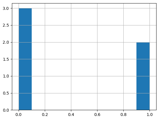
print(data.groupby('v1').size().reset_index(name='count'))
# v1 count
# 0 0 4516
# 1 1 653
# feature(v2), label(v1) 분리
xdata = data['v2']
ydata = data['v1']
print(xdata[:3])
# 0 Go until jurong point, crazy.. Available only ...
# 1 Ok lar... Joking wif u oni...
# 2 Free entry in 2 a wkly comp to win FA Cup fina...
print(ydata[:3])
# 0 0
# 1 0
# 2 1
- token 처리
from tensorflow.keras.preprocessing.text import Tokenizer
tok = Tokenizer()
tok.fit_on_texts(xdata)
print(tok.word_index) # {'i': 1, 'to': 2, 'you': 3, 'a': 4, 'the': 5, 'u': 6, 'and': 7, 'in': 8, 'is': 9, 'me': 10 ...
sequences = tok.texts_to_sequences(xdata)
print(xdata[:5])
# 0    Go until jurong point, crazy.. Available only ...
# 1                        Ok lar... Joking wif u oni...
# 2    Free entry in 2 a wkly comp to win FA Cup fina...
# 3    U dun say so early hor... U c already then say...
# 4    Nah I don't think he goes to usf, he lives aro...
print(sequences[:5])
# [[47, 433, 4013, 780, 705, 662, 64, 8, 1202, 94, 121, 434, 1203, ...
word_index = tok.word_index
print(word_index)
# {'i': 1, 'to': 2, 'you': 3, 'a': 4, 'the': 5, 'u': 6, 'and': 7, 'in': 8, 'is': 9, 'me': 10, ...
print(len(word_index)) # 8920
# 전체 자료 중 등장빈도 수, 비율 확인
threshold = 2                   # 등장빈도 수를 제한
total_count = len(word_index)   # 전체 단어 수
rare_count = 0                  # 빈도 수가 threshold 보다 작은 경우
total_freq = 0                  # 전체 단어 빈도 수 총합 비율
rare_freq = 0                   # 빈도 수 가 threshold보다 작은 경우의 단어 빈도 수 총합 비율 전체 자료 중 등장빈도 수, 비율 확인
threshold = 2                   # 등장빈도 수를 제한
total_count = len(word_index)   # 전체 단어 수
rare_count = 0                  # 빈도 수가 threshold 보다 작은 경우
total_freq = 0                  # 전체 단어 빈도 수 총합 비율
rare_freq = 0                   # 빈도 수 가 threshold보다 작은 경우의 단어 빈도 수 총합 비율

# dict type의 단어/빈도수 얻기
for key, value in tok.word_counts.items():
    #print('k:{} va:{}'.format(key, value))
    # k:jd va:1
    # k:accounts va:1
    # k:executive va:2
    # k:parents' va:2
    # k:picked va:7
    # k:downstem va:1
    # k:08718730555 va:
    total_freq = total_freq + value

    if value < threshold:
        rare_count = rare_count + 1
        rare_freq = rare_freq + value

print('등장빈도가 1회인 단어 수 :', rare_count)                                # 등장빈도가 1회인 단어 수 : 4908
print('등장빈도가 1회인 단어 비율 :', (rare_count / total_count) * 100)        # 등장빈도가 1회인 단어 비율 : 55.02242152466368
print('전체 중 등장빈도가 1회인 단어 비율 :', (rare_freq / total_freq) * 100)  # 전체 중 등장빈도가 1회인 단어 비율 : 6.082538108811501

tok = Tokenizer(num_words= total_count - rare_count + 1)
vocab_size = len(word_index) + 1
print('단어 집합 크기 :', vocab_size)   # 단어 집합 크기 : 8921

# train/test 8:2
n_of_train = int(len(sequences) * 0.8)
n_of_test = int(len(sequences) - n_of_train)
print('train lenghth :', n_of_train)    # train lenghth : 4135
print('test lenghth :', n_of_test)      # test lenghth : 1034

# 메일의 길이 확인
x_data = sequences
print('메일의 최대 길이 :', max((len(i) for i in x_data)))          # 메일의 최대 길이 : 189
print('메일의 평균 길이 :', (sum(map(len, x_data)) / len(x_data)))  # 메일의 평균 길이 : 15.610369510543626

# 시각화
import matplotlib.pyplot as plt
plt.hist([len(siz) for siz in x_data], bins=50)
plt.xlabel('length')
plt.ylabel('count')
plt.show()
from tensorflow.keras.preprocessing.sequence import pad_sequences
max_len = max((len(i) for i in x_data))
data = pad_sequences(x_data, maxlen=max_len)
print(data.shape)       # (5169, 189)

# train/test 분리
import numpy as np
x_train = data[:n_of_train]
y_train = np.array(ydata[:n_of_train])
x_test = data[n_of_train:]
y_test = np.array(ydata[n_of_train:])
print(x_train.shape, x_train[:2])   # (4135, 189)
print(y_train.shape, y_train[:2])   # (4135,)
print(x_test.shape, y_test.shape)   # (1034, 189) (1034,)
# 모델
from tensorflow.keras.layers import LSTM, Embedding, Dense, Dropout
from tensorflow.keras.models import Sequential

model = Sequential()
model.add(Embedding(vocab_size, 32))
model.add(LSTM(32, activation='tanh'))
model.add(Dense(32, activation='relu'))
model.add(Dropout(0.2))
model.add(Dense(1, activation='sigmoid'))
print(model.summary())      # Total params: 294,881

model.compile(optimizer='adam', loss='binary_crossentropy', metrics=['acc'])
history = model.fit(x_train, y_train, epochs=5, batch_size=32, validation_split=0.25, verbose=2)
print('loss, acc :', model.evaluate(x_test, y_test))    # loss, acc : [0.05419406294822693, 0.9893617033958435]

# print(x_test[0])
word_index = reuters.get_word_index()
print(word_index)       # {'mdbl': 10996, 'fawc': 16260, 'degussa': 12089, 'woods': 8803, 'hanging': 13796, ... }

index_to_word = {}
for k, v in word_index.items():
    index_to_word[v] = k

print(index_to_word)    # {10996: 'mdbl', 16260: 'fawc', 12089: 'degussa', 8803: 'woods', 13796: 'hanging ... }
print(index_to_word[1]) # the
print(index_to_word[10])    # for
print(index_to_word[100])   # group

print(x_train[0])                                       # [1, 2, 2, 8, 43, 10, 447, 5, 25, 207, 270, 5, 2, 111, 16, 369, ...
print(' '.join(index_to_word[i] for i in x_train[0]))   # he of of mln loss for plc said at only ended said of  ...
len_result = [len(s) for s in x_train]
print('리뷰 최대 길이 :', np.max(len_result))  # 2494
print('리뷰 평균 길이 :', np.mean(len_result)) # 238.71364

plt.subplot(1, 2, 1)
plt.boxplot(len_result)
plt.subplot(1, 2, 2)
plt.hist(len_result, bins=50)
plt.show()
word_to_index = imdb.get_word_index()
index_to_word = {}
for k, v in word_to_index.items():
    index_to_word[v] = k
print(index_to_word)        # {34701: 'fawn', 52006: 'tsukino', 52007: 'nunnery', 16816: 'sonja', ...
print(index_to_word[1])     # the
print(index_to_word[1408])  # woods

print(x_train[0])           # [1, 14, 22, 16, 43, 530, 973, 1622, ...
print(y_train[0])           # 1
print(' '.join([index_to_word[index] for index in x_train[0]]))     # the as you with out themselves powerful lets loves their ...
from tensorflow.keras.layers import Conv1D, GlobalMaxPooling1D, MaxPooling1D, Dropout

model = Sequential()
model.add(Embedding(vocab_size, 256))
model.add(Conv1D(256, kernel_size=3, padding='valid', activation='relu', strides=1))
model.add(GlobalMaxPooling1D())
model.add(Dense(1, activation='sigmoid'))
print(model.summary())          # Total params: 2,757,121

model.compile(loss='binary_crossentropy', optimizer='adam', metrics=['acc'])
es = EarlyStopping(monitor='val_loss', mode='auto', patience=3, baseline=0.01)
ms = ModelCheckpoint('tfrmm12_1.h5', monitor='val_acc', mode='max', save_best_only = True)
history = model.fit(x_train, y_train, validation_data=(x_test, y_test), epochs=100, batch_size=64, verbose=2, callbacks=[es, ms])

loaded_model = load_model('tfrmm12_1.h5')
print('acc :',loaded_model.evaluate(x_test, y_test)[1])     # acc : 0.8984400033950806
print('loss :',loaded_model.evaluate(x_test, y_test)[0])    # loss : 0.24771703779697418
- 시각화
vloss = history.history['val_loss']
loss = history.history['loss']
x_len = np.arange(len(loss))
plt.plot(x_len, vloss, marker='+', c='black', label='val_loss')
plt.plot(x_len, loss, marker='s', c='red', label='loss')
plt.legend()
plt.grid()
plt.show()

import re
def sentiment_predict(new_sentence):
  new_sentence = re.sub('[^0-9a-zA-Z ]', '', new_sentence).lower()

  # 정수 인코딩
  encoded = []
  for word in new_sentence.split():
    # 단어 집합의 크기를 10,000으로 제한.
    try :
      if word_to_index[word] <= 10000:
        encoded.append(word_to_index[word]+3)
      else:
        encoded.append(2)   # 10,000 이상의 숫자는 <unk> 토큰으로 취급.
    except KeyError:
      encoded.append(2)   # 단어 집합에 없는 단어는 <unk> 토큰으로 취급.

  pad_new = pad_sequences([encoded], maxlen = max_len) # 패딩

  # 예측하기
  score = float(loaded_model.predict(pad_new))
  if(score > 0.5):
    print("{:.2f}% 확률로 긍정!.".format(score * 100))
  else:
    print("{:.2f}% 확률로 부정!".format((1 - score) * 100))
# 99.57% 확률로 긍정!.
# 53.55% 확률로 긍정!.

# 긍/부정 분류 예측
#temp_str = "This movie was just way too overrated. The fighting was not professional and in slow motion."
temp_str = "This movie was a very touching movie."
sentiment_predict(temp_str)

temp_str = " I was lucky enough to be included in the group to see the advanced screening in Melbourne on the 15th of April, 2012. And, firstly, I need to say a big thank-you to Disney and Marvel Studios."
sentiment_predict(temp_str)
#! pip install konlpy

import numpy as np
import pandas as pd
import matplotlib as plt
import re
from konlpy.tag import Okt
from tensorflow.keras.layers import Embedding, Dense, LSTM, Dropout
from tensorflow.keras.models import Sequential, load_model
from tensorflow.keras.callbacks import EarlyStopping, ModelCheckpoint
from tensorflow.keras.preprocessing.text import Tokenizer
from tensorflow.keras.preprocessing.sequence import pad_sequences
drop_train = [index for index, sen in enumerate(x_train) if len(sen) < 1]

x_train = np.delete(x_train, drop_train, axis = 0)
y_train = np.delete(y_train, drop_train, axis = 0)
print(len(x_train), ' ', len(y_train))

print('리뷰 최대 길이 :', max(len(i) for i in x_train))             # 75
print('리뷰 평균 길이 :', sum(map(len, x_train)) / len(x_train))    # 12.169516185172293

plt.hist([len(s) for s in x_train], bins = 50)
plt.show()
- 전체 샘플 중에서 길이가 max_len 이하인 샘플 비율이 몇 % 인지 확인 함수 작성
- IMDB 리뷰 데이터로 감성 분류 : LSTM + Attension (Transformer 기반 기술)
* tf_rnn15_attention.ipynb
# IMDB 리뷰 데이터로 감성 분류 : LSTM + Attension (Transformer 기반 기술)
# 양방향 LSTM과 어텐션 메커니즘(BiLSTM with Attention mechanism)

from tensorflow.keras.datasets import imdb
from tensorflow.keras.utils import to_categorical
from tensorflow.keras.preprocessing.sequence import pad_sequences

vocab_size = 10000
(X_train, y_train), (X_test, y_test) = imdb.load_data(num_words = vocab_size)

print('리뷰의 최대 길이 : {}'.format(max(len(l) for l in X_train)))         # 리뷰의 최대 길이 : 2494
print('리뷰의 평균 길이 : {}'.format(sum(map(len, X_train))/len(X_train)))  # 리뷰의 평균 길이 : 238.71364

max_len = 500
X_train = pad_sequences(X_train, maxlen=max_len)
X_test = pad_sequences(X_test, maxlen=max_len)

...
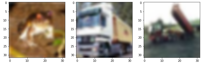
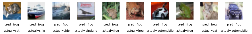
fig = plt.figure(figsize=(15, 3))
fig.subplots_adjust(hspace = 0.4, wspace = 0.4)

for i, idx in enumerate(range(len(x_test[:10]))):
    img = x_test[idx]
    ax = fig.add_subplot(1, len(x_test[:10]), i+1)
    ax.axis('off')
    ax.text(0.5, -0.35, 'pred=' + str(pred_single[idx]),\
            fontsize=10, ha = 'center', transform = ax.transAxes)
    ax.text(0.5, -0.7, 'actual=' + str(actual_single[idx]),\
            fontsize=10, ha = 'center', transform = ax.transAxes)
    ax.imshow(img)

plt.show()
- CNN + DENSE 레이어로만 분류작업2
import numpy as np
import matplotlib.pyplot as plt
from tensorflow.keras.layers import Input, Flatten, Dense, Conv2D, Activation, BatchNormalization, ReLU, LeakyReLU, MaxPool2D
from tensorflow.keras.models import Sequential, Model
from tensorflow.keras.optimizers import Adam
from tensorflow.keras.utils import to_categorical
from tensorflow.keras.datasets import cifar10
input_layer = Input(shape=(32,32,3))
x = Conv2D(filters=64, kernel_size=3, strides=2, padding='same')(input_layer)
x = MaxPool2D(pool_size=(2,2))(x)
#x = ReLU(x)
x = BatchNormalization()(x)
x = LeakyReLU()(x)

x = Conv2D(filters=64, kernel_size=3, strides=2, padding='same')(x)
x = MaxPool2D(pool_size=(2,2))(x)
x = BatchNormalization()(x)
x = LeakyReLU()(x)

x = Flatten()(x)

x = Dense(512)(x)
x = BatchNormalization()(x)
x = LeakyReLU()(x)

x = Dense(128)(x)
x = BatchNormalization()(x)
x = LeakyReLU()(x)

x = Dense(NUM_CLASSES)(x)
output_layer = Activation('softmax')(x)

model = Model(input_layer, output_layer)
import tensorflow as tf

from tensorflow.keras.models import Sequential
from tensorflow.keras.layers import Dense, Conv2D, Flatten, Dropout, MaxPooling2D
from tensorflow.keras.preprocessing.image import ImageDataGenerator

import os
import numpy as np
import matplotlib.pyplot as plt
train_dir = os.path.join(PATH, 'train')
validation_dir = os.path.join(PATH, 'validation')

train_cats_dir = os.path.join(train_dir, 'cats')  # directory with our training cat pictures
train_dogs_dir = os.path.join(train_dir, 'dogs')  # directory with our training dog pictures
validation_cats_dir = os.path.join(validation_dir, 'cats')  # directory with our validation cat pictures
validation_dogs_dir = os.path.join(validation_dir, 'dogs')  # directory with our validation dog pictures
- 이미지를 확인
num_cats_tr = len(os.listdir(train_cats_dir))
num_dogs_tr = len(os.listdir(train_dogs_dir))
# num_cats_te = len(os.listdir(test_cats_dir))
# num_dogs_te = len(os.listdir(test_dogs_dir))

num_cats_val = len(os.listdir(validation_cats_dir))
num_dogs_val = len(os.listdir(validation_dogs_dir))

total_train = num_cats_tr + num_dogs_tr
total_val = num_cats_val + num_dogs_val
# total_te = num_cats_te + num_dogs_te

print('total training cat images:', num_cats_tr)
print('total training dog images:', num_dogs_tr)
# print('total test dog images:', total_te)
# total training cat images: 1000
# total training dog images: 1000

print('total validation cat images:', num_cats_val)
print('total validation dog images:', num_dogs_val)
# total validation cat images: 500
# total validation dog images: 500
print("--")
print("Total training images:", total_train)
print("Total validation images:", total_val)
# Total training images: 2000
# Total validation images: 1000
- ImageDataGenerator
train_image_generator = ImageDataGenerator(rescale=1./255) # Generator for our training data
validation_image_generator = ImageDataGenerator(rescale=1./255) # Generator for our validation data

train_data_gen = train_image_generator.flow_from_directory(batch_size=batch_size,
                                                           directory=train_dir,
                                                           shuffle=True,
                                                           target_size=(IMG_HEIGHT, IMG_WIDTH),
                                                           class_mode='binary')
val_data_gen = validation_image_generator.flow_from_directory(batch_size=batch_size,
                                                              directory=validation_dir,
                                                              target_size=(IMG_HEIGHT, IMG_WIDTH),
                                                              class_mode='binary')
4. 데이터 확인
sample_training_images, _ = next(train_data_gen)

# This function will plot images in the form of a grid with 1 row and 5 columns where images are placed in each column.
def plotImages(images_arr):
    fig, axes = plt.subplots(1, 5, figsize=(20,20))
    axes = axes.flatten()
    for img, ax in zip( images_arr, axes):
        ax.imshow(img)
        ax.axis('off')
    plt.tight_layout()
    plt.show()

plotImages(sample_training_images[:5])
image_gen = ImageDataGenerator(rescale=1./255, horizontal_flip=True)
train_data_gen = image_gen.flow_from_directory(batch_size=batch_size,
                                               directory=train_dir,shuffle=True,
                                               target_size=(IMG_HEIGHT, IMG_WIDTH))
augmented_images = [train_data_gen[0][0][0] for i in range(5)]

# Re-use the same custom plotting f
image_gen = ImageDataGenerator(rescale=1./255, horizontal_flip=True)
train_data_gen = image_gen.flow_from_directory(batch_size=batch_size,
                                               directory=train_dir,
                                               shuffle=True,
                                               target_size=(IMG_HEIGHT, IMG_WIDTH))

augmented_images = [train_data_gen[0][0][0] for i in range(5)]

# Re-use the same custom plotting function defined and used
# above to visualize the training images
plotImages(augmented_images)
전부 적용
image_gen_train = ImageDataGenerator(
                    rescale=1./255,
                    rotation_range=45,
                    width_shift_range=.15,
                    height_shift_range=.15,
                    horizontal_flip=True,
                    zoom_range=0.5
                    )

train_data_gen = image_gen_train.flow_from_directory(batch_size=batch_size,
                                                     directory=train_dir,
                                                     shuffle=True,
                                                     target_size=(IMG_HEIGHT, IMG_WIDTH),
                                                     class_mode='binary')

augmented_images = [train_data_gen[0][0][0] for i in range(5)]
plotImages(augmented_images)
! ls -al
! pip install tensorflow-datasets
import os
import numpy as np
import matplotlib.pyplot as plt
import tensorflow as tf
import tensorflow_datasets as tfds
전이 학습 파이 튜닝 : 미리 학습된 ConvNet의 마지막 FC Layer만 변경해 분류 실행
이전 학습의 모바일넷을 동경시키고 새로 추가한 레이어만 학습 (베이스 모델의 후방 레이어 일부만 다시 학습)
먼저 베이스 모델을 동결한 후 학습 진행 -> 학습이 끝나면 동결 해제
base_model.trainable = True
print('베이스 모델의 레이어 :', len(base_model.layers)) # 베이스 모델의 레이어 : 154

fine_tune_at = 100

for layer in base_model.layers[:fine_tune_at]:
    layer.trainable = False
pwd						: 사용자의 경로
ls						: 디렉토리
-l						: 자세히 보기
-a						: 숨김파일 확인
-al						: 숨김파일 자세히 보기
~						: 현재 사용자의 경로
/						: 리눅스의 경로
vi aaa					: 파일 생성
esc						: 입력어 대기화면
i, a					: append
shift + space			: 한영
:q!						: 미저장 종료
:wq						: 저장 후 종료
vi bbb.txt				: 파일 생성
리눅스에선 확장자 X
vi .ccc					: 숨김 파일 생성
.						: 숨김 파일
yy		  				: 복사
p 		  				: 붙여넣기
dd        				: 한줄 지우기
숫자+명령어   				: 명령어 여러번 반복
:set nu   				: 줄 번호 넣기
:set nonu 				: 줄 번호 제거
whoami    				: id 확인
s /home					: id 확인
mkdir kbs 				: 디렉토리 생성
mkdir -p  mbc/sbs 		: 상위 디렉토리 자동 생성
cd 디렉토리명 				: 디렉토리 변경
cd ~  					: home으로
cd .. 					: 상위 디렉토리로 이동
rmdir 디렉토리명   			: 디렉토리 삭제
rm 파일명         			: 파일 삭제
rm -rf kbs      		: 파일 있어도 삭제 가능
touch 파일명      			: 빈 파일 생성
cat 파일명        			: 파일 내용 확인
cat 파일명1 파일명2 			: 파일 내용확인
cp 파일명 디렉토리명/ 			: 파일 복사
cp 파일명 디렉토리명/새파일명 	: rename 파일 복사
mv 파일명 디렉토리        	: 파일 이동
rename 파일명 happy 새파일명 : 파일명 변경
mv 파일명 새파일명 			: 파일명 변경
head -3 파일명 			: 앞에 3줄 확인
tail -3 파일명 			: 뒤에 3줄 확인
more +10 파일명 			:
grep "검색어" 파일명 		: 검색
grep "[^A-Z]" 파일명* 		: 해당 파일명을 가진 모든 파일에서 대문자가 아닌 값 검색
whereis java 			: 파일 설치 모든 경로
whichis java 			: 파일 설치 경로
ifconfig				: ip 확인
su - root				: super user 접속
su - hadoop				: hadoop 일반 계정에 접속
useradd tom				: tom 일반 계정 만들기
passwd tom				: tom 일반 계정에 암호설정
exit					: 해당 계정 logout
userdel james			: 계정 삭제(logout상태에서)
rm -rf james			: 잔여 계정목록 삭제
-rwxrw-r--				: user, group, others
chmod u-w test.txt		: 현재 사용자에게 쓰기 권한 제거
chmod u-r test.txt		: 현재 사용자에게 읽기 권한 제거
chmod u+rwx test. extxt	: 현재 사용자에게 읽기/쓰기/excute 권한 추가
./test.txt				: 명령어 실행
chmod 777 test.txt		: 모든 권한 다 주기
chmod 111 test.txt		: excute 권한 다 주기
ls -l					: 목록 확인
rpm -qa					: 설치 목록확인
rpm -qa java*			: java 설치 경로
yum install gimp		: 설치
su -c 'yum install gimp': 설치
su -c 'yum remove gimp'	: 제거
- gimp 설치
yum list gi*			: 특정단어가 들어간 리스트
which gimp				: gimp 설치 여부 확인
ls -a /usr/bin/gimp
yum info gimp			: 패키지 정보
gimp					: 실행
wget https://t1.daumcdn.net/daumtop_chanel/op/20200723055344399.png : 웹상에서 다운로드
wget https://archive.apache.org/dist/httpd/Announcement1.3.txt		: 웹상에서 다운로드
- 파일 압축
vi aa
gzip aa					: 압축
gzip -d aa.gz			: 압축해제
bzip2 aa				: 압축
bzip2 -d aa.bz2			: 압축해제
tar cvf	my.tar aa bb	: 파일 묶기
tar xvf my.tar			: 압축 해제
java -version			: 자바 버전 확인
su -					: 관리자 접속
yum update				: 패키지 업데이트
rpm -qa | grep java*	: rpm 사용하여 파일 설치
java					: 자바 실행
javac					: javac 실행
yum remove java-1.8.0-openjdk-headless.x86_64	: 삭제
yum -y install java-11-openjdk-devel			: 패키지 설치
rpm -qa | java			: 설치 확인
- 이클립스 다운로드
mkdir work				: 디렉토리 생성
cd work
eclipse.org - download - 탐색기 - 다운로드 - 복사 - work 붙여넣기
tar xvfz eclipse tab키	: 압축해제
cd eclipse/
./eclipse
work -> jsou
open spective - java
Gerneral - Workspace - utf-8
Web  - utf-8
file - new - java project - pro1 / javaSE-11 - Don't create
new - class - test / main
sysout alt /
sum inss
apache.org 접속
맨아래 Tomcat 클릭
Download / Tomcat 10 클릭
tar.gz (pgp, sha512) 다운로드
터미널 창 접속
ls /~다운로드
cd work
mv ~/다운로드.apach ~~ .gz ./
tar xvfz apache-tomcat-10.0.5.tar.gz
cd apache-tomcat-10.0.5/
cd bin/
pwd
./startup.sh							: 서버 실행
http://localhost:8080/ 접속
./shutdown.sh							: 서버 종료
./catalina.sh run						: 개발자용 서버 실행
http://localhost:8080/ 접속
ctrl + c								: 개발자용 서버 종료
cd conf
ls se*
vi server.xml
cd ~
pwd
eclipse 접속
Dynimic web project 생성
이름 : webpro / Targert runtime -> apache 10 및 work - apache 폴더 연결
webapp에 abc.html 생성.
window - web browser - firefox
내용 작성 후 서버 실행.
install.packages("ggplot2")
library(ggplot2)
a <- 10
print(a)
print(head(iris, 3))
ggplot(data=iris, aes(x = Petal.Length, y = Petal.Width)) + geom_point()
- R studio 서버
vi /etc/selinux/config
SELINUX=permissive으로 수정
reboot
su - root
vi /etc/selinux/config
cd /usr/lib/firewalld/services/
ls http*
cp http.xml R.xml
vi R.xml
port="8787"으로 수정
firewall-cmd --permanent --zone=public --add-service=R
firewall-cmd --reload
https://www.rstudio.com/products/rstudio/download-server/
redhat/centos
wget https://download2.rstudio.org/server/centos7/x86_64/rstudio-server-rhel-1.4.1106-x86_64.rpm
wget https://download2.rstudio.org/server/fedora28/x86_64/rstudio-server-rhel-1.2.5033-x86_64.rpm

yum install --nogpgcheck rstudio-server-rhel-1.4.1106-x86_64.rpm
systemctl status rstudio-server
systemctl start rstudio-server
http://ip addr:8787/auth-sign-in	: 본인 ip에 접속

useradd testuser
passwd testuser
ls /home

mkdir mbc
cd mbc
ls
Download - Linux / 64-Bit (x86) Installer (529 MB) - 링크주소 복사
wget https://repo.anaconda.com/archive/Anaconda3-2020.02-Linux-x86_64.sh
chmod +x Anaconda~~
./Anaconda~~
q
yes
vi .bash_profile		: 파일 수정
=============================================
PATH=$PATH:$HOME/bin
export PATH

# added by Anaconda3 installer
export PATH="/home/hadoop/anaconda3/bin:$PATH"
==============================================
source .bash_profile
python3
conda deactivate     : 가상환경 나오기
source activate base : 가상환경 들어가기
jupyter notebook
jupyter lab
localhost:8888/tree
ctrl + c
y
jupyter notebook --generate-config
python
from notebook.auth import passwd
passwd()     #sha1 값 얻기
quit()
비밀번호 설정
Verify password 복사
vi .jupyter/jupyter_notebook_config.py		: 파일 수정
ctrl + end
==============================================
c.NotebookApp.password =u'       Verify password 붙여넣기		'
==============================================
quit()
vi .jupyter/jupyter_notebook_config.py
su -
cd /usr/lib/firewalld/services/
cp http.xml NoteBook.xml
vi NoteBook.xml
8001포트 설정
:wq
systemctl status firewalld.service           방화벽 서비스 상태 확인  start, stop, enable
firewall-cmd --permanent --zone=public --add-service=NoteBook
firewall-cmd --reload
jupyter notebook --ip=0.0.0.0 --port=8001 --allow-root
jupyter lab --ip=0.0.0.0 --port=8001 --allow-root
vi .jupyter/jupyter_notebook_config.py
==============================================
c.NotebookApp.open_browser = False
==============================================
conda deactivate	: 가상환경 나오기
java -version		: 자바 버전 확인
ls -al /etc/alternatives/java	: 자바 경로 확인 후 경로 복사
 => /usr/ ~~ .x86_64 복사
https://apache.org/ 접속 => 맨 밑에 hadoop접속 => Download =>
su -				: 관리자 접속
cd /usr/lib/firewalld/services/	: 특정 port 방화벽 해제
cp http.xml hadoop.xml
vi hadoop.xml					: 파일 수정 후 저장(:wq)
==============================================
<?xml version="1.0" encoding="utf-8"?>
<service>
    <short>Hadoop</short>
    <description></description>
    <port protocol="tcp" port="8042"/>
    <port protocol="tcp" port="9864"/>
    <port protocol="tcp" port="9870"/>
    <port protocol="tcp" port="8088"/>
    <port protocol="tcp" port="19888"/>
</service>
==============================================
firewall-cmd --permanent --zone=public --add-service=hadoop
firewall-cmd --reload
exit
wget http://apache.mirror.cdnetworks.com/hadoop/common/hadoop-3.2.1/hadoop-3.2.1.tar.gz
tar xvzf hadoop-3.2.1.tar.gz
vi .bash_profile
==============================================
# User specific environment and startup programs
export JAVA_HOME=/usr/ ~~ .x86_64 붙여넣기
export HADOOP_HOME=/home/사용자명/hadoop-3.2.1
PATH=$PATH:$HOME/.local/bin:$HOME/bin:$HADOOP_HOME/bin:$HADOOP_HOME/sbin  #추가
export PATH
==============================================
source .bash_profile		: .bash_profile을 수정된 내용으로 등록
conda deactivate
ls
cd hadoop-3.2.1/
vi README.txt
vi kor.txt					: 임의 내용 입력
cd etc
cd hadoop
pwd
vi hadoop-env.sh			: 파일 상단에 입력
==============================================
export JAVA_HOME=/usr/ ~~ .x86_64 붙여넣기
==============================================

vi core-site.xml        : 하둡 공통 설정을 기술
==============================================
<configuration>
        <property>
                <name>fs.default.name</name>
                <value>hdfs://localhost:9000</value>
        </property>
      <property>
                 <name>hadoop.tmp.dir</name>
                       <value>/home/사용자명/hadoop-3.2.1/tmp/</value>
            </property>
</configuration>
==============================================

vi hdfs-site.xml      : HDFS 동작에 관한 설정
==============================================
<configuration>
     <property>
          <name>dfs.replication</name>
          <value>1</value>
     </property>
</configuration>
==============================================

vi yarn-env.sh         : yarn 설정 파일
==============================================
export JAVA_HOME=/usr/ ~~ .x86_64 붙여넣기
==============================================

vi mapred-site.xml      : yarn 설정 파일
==============================================
<configuration>
     <property>
          <name>mapreduce.framework.name</name>
          <value>yarn</value>
     </property>
     <property>
        <name>mapreduce.admin.user.env</name>
        <value>HADOOP_MAPRED_HOME=$HADOOP_COMMON_HOME</value>
    </property>
    <property>
        <name>yarn.app.mapreduce.am.env</name>
        <value>HADOOP_MAPRED_HOME=$HADOOP_COMMON_HOME</value>
    </property>
</configuration>
==============================================

vi yarn-site.xml
==============================================
<configuration>
<!-- Site specific YARN configuration properties -->
     <property>
          <name>yarn.nodemanager.aux-services</name>
          <value>mapreduce_shuffle</value>
     </property>
     <property>
          <name>yarn.nodemanager.aux-services.mapreduce.shuffle.class</name>
          <value>org.apache.hadoop.mapred.ShuffleHandler</value>
     </property>
</configuration>
==============================================

cd					: root로 이동
hdfs namenode -format
hadoop version		: 하둡 버전 확인

ssh					: 원격지 시스템에 접근하여 암호화된 메시지를 전송할 수 있는 프로그램
ssh-keygen -t rsa	: ssh 키 생성. enter 3번.
cd .ssh
scp id_rsa.pub /home/사용자명/.ssh/authorized_keys	: 생성키를 접속할 때 사용하도록 복사함. yes
ssh 사용자명@localhost

start-all.sh		: deprecated
start-dfs.sh
start-yarn.sh
mr-jobhistory-daemon.sh start historyserver	: 안해도됨

jps					: 하둡 실행 상태 확인 - NameNode와 DataNode의 동작여부 확인

stop-all.sh			: deprecated
stop-dfs.sh
stop-yarn.sh
http://localhost:9870/ 접속 : Summary(HDFS 상태 확인) http://localhost:8088/ 접속 : All Applications
conda deactivate
start-dfs.sh
start-yarn.sh
jps
http://localhost:9870/ 접속	: Summary(HDFS 상태 확인)
http://localhost:8088/ 접속	: All Applications
eclipse 실행
import java.io.IOException;
import java.util.StringTokenizer;

import org.apache.hadoop.conf.Configuration;
import org.apache.hadoop.fs.Path;
import org.apache.hadoop.io.IntWritable;
import org.apache.hadoop.io.Text;
import org.apache.hadoop.mapreduce.Job;
import org.apache.hadoop.mapreduce.Mapper;
import org.apache.hadoop.mapreduce.Reducer;
import org.apache.hadoop.mapreduce.lib.input.FileInputFormat;
import org.apache.hadoop.mapreduce.lib.output.FileOutputFormat;

public class WordCount {

  public static class TokenizerMapper
       extends Mapper<Object, Text, Text, IntWritable>{

    private final static IntWritable one = new IntWritable(1);
    private Text word = new Text();

    public void map(Object key, Text value, Context context
                    ) throws IOException, InterruptedException {
      StringTokenizer itr = new StringTokenizer(value.toString());
      while (itr.hasMoreTokens()) {
        word.set(itr.nextToken());
        context.write(word, one);
      }
    }
  }

  public static class IntSumReducer
       extends Reducer<Text,IntWritable,Text,IntWritable> {
    private IntWritable result = new IntWritable();

    public void reduce(Text key, Iterable<IntWritable> values,
                       Context context
                       ) throws IOException, InterruptedException {
      int sum = 0;
      for (IntWritable val : values) {
        sum += val.get();
      }
      result.set(sum);
      context.write(key, result);
    }
  }

  public static void main(String[] args) throws Exception {
    Configuration conf = new Configuration();

	conf.set("fs.default.name", "hdfs://localhost:9000");

    Job job = Job.getInstance(conf, "word count");
    job.setJarByClass(WordCount.class);
    job.setMapperClass(TokenizerMapper.class);
    job.setCombinerClass(IntSumReducer.class);
    job.setReducerClass(IntSumReducer.class);
    job.setOutputKeyClass(Text.class);
    job.setOutputValueClass(IntWritable.class);

    FileInputFormat.addInputPath(job, new Path("hdfs://localhost:9000/test/data.txt"));
    FileOutputFormat.setOutputPath(job, new Path("hdfs://localhost:9000/out1"));
	System.out.println("success");

    //FileInputFormat.addInputPath(job, new Path(args[0]));
    //FileOutputFormat.setOutputPath(job, new Path(args[1]));

	System.exit(job.waitForCompletion(true) ? 0 : 1);
  }
}
ls
cd hadoop-3.2.1/
vi data.txt
임의 텍스트 입력
hdfs dfs -put data.txt /test
hdfs dfs -get /out1/part* result1.txt
vi result1.txt
vi vote.txt
임의 텍스트 입력
hdfs dfs -put vote.txt /test
src - new - class - pack2.VoteMapper
* VoteMapper.java
import java.util.regex.*;
import org.apache.hadoop.io.IntWritable
import org.apache.hadoop.io.Text
import org.apache.hadoop.mapreduce.Mapper


public class VoteMapper extends Mapper<Object, Text, Text, IntWritable>{
	private final static IntWritable one =  new IntWritable(1);
	private Text word = new Text();

	@Override
	public void map(Object ket, Text value, Context context)throws IOException, InterruptedException{
		String str = value.toString();
		System.out.println(str);
		String regex = "홍길동|신기해|한국인";
		Pattern pattern = Pattern.compile(regex);
		Matcher matcher = pattern.matcher(str);
		String result = "";
		while(match.find()){
			result += matcher.group() + "";
		}
		StringTokenizer itr = new StringTokenizer(result);

		while(itr.hasMoreTokens()){
			word.set(itr.nextToken());
			context.write(word, one);
		}
	}
}
src - new - class - pack2.VoteReducer
* VoteReducer.java
public class VoteReducer extends Reducer<Textm IntWritable, Text, IntWritable>{
	private IntWritable result = new IntWritable();

	@Override
	public void reduce(Text key, Iterable<IntWritable> values, Context context) throw IOException, InterruptedException{
		int sum = 0;
		for(IntWritable val:values){
			sum += val.get();
		}

		result.set(sum);
		context.wrtie(key, result);
	}
}
src - new - class - pack2.VoteCount
* VoteCount.java
public class VoteCount{
	public static void main(String[] args) throws Exception{
		Configuration conf = new Configuration();
		conf.set("fs.default.name", "hdfs://localhost:9000");

		Job job = Job.getInstance(conf, "vote");
		job.setJarByClass(VoteCount.class);
		job.setMapperClass(VoteMapper.class);
		job.setCombinerClass(VoteReducer.class);
		job.setReducerClass(VoteReducer.class);
		job.setOutputKeyClass(Text.class);
		job.setOutputValueClass(IntWritable.class);

		FileInputFormat.addInputPath(job, new Path("hdfs://localhost:9000/test/vote.txt"));
		FileOutputFormat.setOutputPath(job, new Path("hdfs://localhost:9000/out2"));

		System.out.println("end");

		System.exit(job.waitForCompletion(true)?0:1);
	}
}
import tensorflow.compat.v1 as tf # tf2.x 환경에서 1.x 소스 실행 시
tf.disable_v2_behavior() # tf2.x 환경에서 1.x 소스 실행 시
x_data = [[1,2],[2,3],[3,4],[4,3],[3,2],[2,1]]
y_data = [[0],[0],[0],[1],[1],[1]]
# placeholders for a tensor that will be always fed.
X = tf.placeholder(tf.float32, shape=[None, 2])
Y = tf.placeholder(tf.float32, shape=[None, 1])
W = tf.Variable(tf.random_normal([2, 1]), name='weight')
b = tf.Variable(tf.random_normal([1]), name='bias')
# Hypothesis using sigmoid: tf.div(1., 1. + tf.exp(tf.matmul(X, W)))
hypothesis = tf.sigmoid(tf.matmul(X, W) + b)
# 로지스틱 회귀에서 Cost function 구하기
cost = -tf.reduce_mean(Y * tf.log(hypothesis) + (1 - Y) * tf.log(1 - hypothesis))
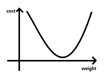
# Optimizer(코스트 함수의 최소값을 찾는 알고리즘) 구하기
train = tf.train.GradientDescentOptimizer(learning_rate=0.01).minimize(cost)
predicted = tf.cast(hypothesis > 0.5, dtype=tf.float32)
accuracy = tf.reduce_mean(tf.cast(tf.equal(predicted, Y), dtype=tf.float32))
with tf.Session() as sess:
sess.run(tf.global_variables_initializer())
for step in range(10001):
cost_val, _ = sess.run([cost, train], feed_dict={X: x_data, Y: y_data})
if step % 200 == 0:
print(step, cost_val)
# Accuracy report (정확도 출력)
h, c, a = sess.run([hypothesis, predicted, accuracy],feed_dict={X: x_data, Y: y_data})
print("\nHypothesis: ", h, "\nCorrect (Y): ", c, "\nAccuracy: ", a)
import tensorflow.compat.v1 as tf
tf.disable_v2_behavior() : 텐서플로우 2환경에서 1 소스 실행 시 사용
import numpy as np
from tensorflow.keras.models import Sequential
from tensorflow.keras.layers import Dense, Activation

np.random.seed(0)

x = np.array([[1,2],[2,3],[3,4],[4,3],[3,2],[2,1]])
y = np.array([[0],[0],[0],[1],[1],[1]])

model = Sequential([
    Dense(units = 1, input_dim=2),  # input_shape=(2,)
    Activation('sigmoid')
])

model.compile(loss='binary_crossentropy', optimizer='adam', metrics=['accuracy'])

model.fit(x, y, epochs=1000, batch_size=1, verbose=1)

meval = model.evaluate(x,y)
print(meval)            # [0.209698(loss),  1.0(정확도)]

pred = model.predict(np.array([[1,2],[10,5]]))
print('예측 결과 : ', pred)     # [[0.16490099] [0.9996613 ]]
print('예측 결과 : ', np.squeeze(np.where(pred > 0.5, 1, 0)))  # [0 1]

for i in pred:
    print(1 if i > 0.5 else print(0))
print([1 if i > 0.5 else 0 for i in pred])
# 2. function API 사용
from tensorflow.keras.layers import Input
from tensorflow.keras.models import Model

inputs = Input(shape=(2,))
outputs = Dense(1, activation='sigmoid')
model2 = Model(inputs, outputs)

model2.compile(loss='binary_crossentropy', optimizer='adam', metrics=['accuracy'])

model2.fit(x, y, epochs=500, batch_size=1, verbose=0)

meval2 = model2.evaluate(x,y)
print(meval2)            # [0.209698(loss),  1.0(정확도)]
# 과적합 방지 - train/test
x_train, x_test, y_train, y_test = train_test_split(x, y, test_size=0.3, random_state=12)
print(x_train.shape, x_test.shape, y_train.shape)     # (4547, 12) (1950, 12) (4547,)

# model
model = Sequential()
model.add(Dense(30, input_dim=12, activation='relu'))
model.add(tf.keras.layers.BatchNormalization()) # 배치정규화. 그래디언트 손실과 폭주 문제 개선
model.add(Dense(15, activation='relu'))
model.add(tf.keras.layers.BatchNormalization()) # 배치정규화. 그래디언트 손실과 폭주 문제 개선
model.add(Dense(8, activation='relu'))
model.add(tf.keras.layers.BatchNormalization()) # 배치정규화. 그래디언트 손실과 폭주 문제 개선
model.add(Dense(1, activation='sigmoid'))
print(model.summary()) # Total params: 992

# 학습 설정
model.compile(optimizer='adam', loss='binary_crossentropy', metrics=['accuracy'])

# 모델 평가
loss, acc = model.evaluate(x_train, y_train, verbose=2)
print('훈련되지않은 모델의 분류 정확도 :{:5.2f}%'.format(100 * acc))  # 훈련되지않은 모델의 평가 :25.14%
model.add(tf.keras.layers.BatchNormalization()) : 배치정규화. 그래디언트 손실과 폭주 문제 개선
# 모델 저장 및 폴더 설정
import os
MODEL_DIR = './model/'
if not os.path.exists(MODEL_DIR): # 폴더가 없으면 생성
    os.mkdir(MODEL_DIR)

# 모델 저장조건 설정
modelPath = "model/{epoch:02d}-{loss:4f}.hdf5"

# 모델 학습 시 모니터링의 결과를 파일로 저장
chkpoint = ModelCheckpoint(filepath='./model/abc.hdf5', monitor='loss', save_best_only=True)
#chkpoint = ModelCheckpoint(filepath=modelPath, monitor='loss', save_best_only=True)

# 학습 조기 종료
early_stop = EarlyStopping(monitor='loss', patience=5)

# 훈련
# 과적합 방지 - validation_split
history = model.fit(x_train, y_train, epochs=10000, batch_size=64,\
                    validation_split=0.3, callbacks=[early_stop, chkpoint])

model.load_weights('./model/abc.hdf5')
from tensorflow.keras.callbacks import ModelCheckpoint
checkkpoint = ModelCheckpoint(filepath=경로, monitor='loss', save_best_only=True) : 모델 학습 시 모니터링의 결과를 파일로 저장
from tensorflow.keras.callbacks import EarlyStopping
early_stop = EarlyStopping(monitor='loss', patience=5) : 학습 조기 종료
model.fit(x, y, epochs=, batch_size=, validation_split=, callbacks=[early_stop, checkpoint])
'''
여기에서는 인터넷 영화 데이터베이스(Internet Movie Database)에서 수집한 50,000개의 영화 리뷰 텍스트를 담은
IMDB 데이터셋을 사용하겠습니다. 25,000개 리뷰는 훈련용으로, 25,000개는 테스트용으로 나뉘어져 있습니다.
훈련 세트와 테스트 세트의 클래스는 균형이 잡혀 있습니다. 즉 긍정적인 리뷰와 부정적인 리뷰의 개수가 동일합니다.
매개변수 num_words=10000은 훈련 데이터에서 가장 많이 등장하는 상위 10,000개의 단어를 선택합니다.
데이터 크기를 적당하게 유지하기 위해 드물에 등장하는 단어는 제외하겠습니다.
'''

from tensorflow.keras.datasets import imdb
(train_data, train_labels), (test_data, test_labels) = imdb.load_data(num_words=10000)

print(train_data[0])   # 각 숫자는 사전에 있는 전체 문서에 나타난 모든 단어에 고유한 번호를 부여한 어휘사전
# [1, 14, 22, 16, 43, 530, 973, ...

print(train_labels) # 긍정 1 부정0
# [1 0 0 ... 0 1 0]

aa = []
for seq in train_data:
    #print(max(seq))
    aa.append(max(seq))

print(max(aa), len(aa))
# 9999 25000

word_index = imdb.get_word_index() # 단어와 정수 인덱스를 매핑한 딕셔너리
reverse_word_index = dict([(value, key) for (key, value) in word_index.items()])
decord_review = ' '.join([reverse_word_index.get(i - 3, '?') for i in train_data[0]])
print(decord_review)
# ? this film was just brilliant casting location scenery story direction ...
from tensorflow.keras import models, layers, regularizers

model = models.Sequential()
model.add(layers.Dense(16, activation='relu', input_shape=(10000, ), kernel_regularizer=regularizers.l2(0.01)))
# regularizers.l2(0.001) : 가중치 행렬의 모든 원소를 제곱하고 0.001을 곱하여 네트워크의 전체 손실에 더해진다는 의미, 이 규제(패널티)는 훈련할 때만 추가됨
model.add(layers.Dropout(0.3)) # 과적합 방지를 목적으로 노드 일부는 학습에 참여하지 않음
model.add(layers.Dense(16, activation='relu'))
model.add(layers.Dense(1, activation='sigmoid'))

model.compile(optimizer='adam', loss='binary_crossentropy', metrics=['acc'])

print(model.summary())
layers.Dropout(n) : 과적합 방지를 목적으로 노드 일부는 학습에 참여하지 않음
from tensorflow.keras import models, layers, regularizers
x_train, x_test, y_train, y_test = train_test_split(x_scaler, y, test_size=0.3, random_state=1)
n_features = x_train.shape[1] # 열
n_classes = y_train.shape[1]  # 열
print(n_features, n_classes)  # 4 3 => input, output수
- n의 개수 만큼 모델 생성 함수
from tensorflow.keras.models import Sequential
from tensorflow.keras.layers import Dense

def create_custom_model(input_dim, output_dim, out_node, n, model_name='model'):
    def create_model():
        model = Sequential(name = model_name)
        for _ in range(n): # layer 생성
            model.add(Dense(out_node, input_dim = input_dim, activation='relu'))

        model.add(Dense(output_dim, activation='softmax'))
        model.compile(optimizer='adam', loss='categorical_crossentropy', metrics=['acc'])
        return model
    return create_model # 주소 반환(클로저)
models = [create_custom_model(n_features, n_classes, 10, n, 'model_{}'.format(n)) for n in range(1, 4)]
# layer수가 2 ~ 5개 인 모델 생성

for create_model in models:
    print('-------------------------')
    create_model().summary()
    # Total params: 83
    # Total params: 193
    # Total params: 303
- train
history_dict = {}

for create_model in models: # 각 모델 loss, acc 출력
    model = create_model()
    print('Model names :', model.name)
    # 훈련
    history = model.fit(x_train, y_train, batch_size=5, epochs=50, verbose=0, validation_split=0.3)
    # 평가
    score = model.evaluate(x_test, y_test)
    print('test dataset loss', score[0])
    print('test dataset acc', score[1])
    history_dict[model.name] = [history, model]

print(history_dict)
# {'model_1': [<tensorflow.python.keras.callbacks.History object at 0x00000273BA4E7280>, <tensorflow.python.keras.engine.sequential.Sequential object at 0x00000273B9B22A90>], ...}
plt.figure(figsize=(10, 10))
for i in range(25):
plt.subplot(5, 5, i+1)
plt.xticks([])
plt.yticks([])
plt.xlabel(class_names[train_labels[i]])
plt.imshow(train_image[i])
plt.show()
model.save('ke21.h5')
model = tf.keras.models.load_model('ke21.h5')
import pickle
histoy = histoy.history # loss, acc
with open('data.pickle', 'wb') as f: # 파일 저장
pickle.dump(histoy) # 객체 저장
with open('data.pickle', 'rb') as f: # 파일 읽기
history = pickle.load(f) # 객체 읽기
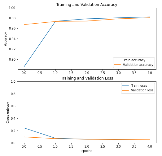
import matplotlib.pyplot as plt
def plot_acc(title = None):
plt.plot(history['accuracy'])
plt.plot(history['val_accuracy'])
if title is not None:
plt.title(title)
plt.ylabel(title)
plt.xlabel('epoch')
plt.legend(['train data', 'validation data'], loc = 0)
plot_acc('accuracy')
plt.show()
def plot_loss(title = None):
plt.plot(history['loss'])
plt.plot(history['val_loss'])
if title is not None:
plt.title(title)
plt.ylabel(title)
plt.xlabel('epoch')
plt.legend(['train data', 'validation data'], loc = 0)
plot_loss('loss')
plt.show()
import tensorflow as tf
from tensorflow.keras.datasets import mnist
from tensorflow.keras.utils import to_categorical
from tensorflow.keras.callbacks import ModelCheckpoint, EarlyStopping
import matplotlib.pyplot as plt
import numpy as np
import sys
import tensorflow as tf
import numpy as np
print(tf.keras.__version__)
1. 데이터 수집 및 가공
x = np.array([[0,0],[0,1],[1,0],[1,1]])
#y = np.array([0,1,1,1]) # or
#y = np.array([0,0,0,1]) # and
y = np.array([0,1,1,0]) # xor : node가 1인 경우 처리 불가
2. 모델 생성(네트워크 구성)
from tensorflow.keras.models import Sequential
from tensorflow.keras.layers import Dense, Activation
model = Sequential([
Dense(input_dim =2, units=1),
Activation('sigmoid')
])
model = Sequential()
model.add(Dense(units=1, input_dim=2))
model.add(Activation('sigmoid'))
# input_dim : 입력층의 뉴런 수
# units : 출력 뉴런 수
from tensorflow.keras.models import Sequential
from tensorflow.keras.layers import Dense, Activation
# 완벽한 모델이라 판단되면 모델을 저장
model.save('test.hdf5')
del model # 모델 삭제
from tensorflow.keras.models import load_model
model2 = load_model('test.hdf5')
pred2 = (model2.predict(x) > 0.5).astype('int32')
print('pred2 :\n', pred2.flatten())
model.save('파일명.hdf5') : 모델 삭제
del model : 모델 삭제
from tensorflow.keras.models import load_model model = load_model('파일명.hdf5') : 모델 불러오기
논리 게이트 XOR 해결을 위해 Node 추가
* ke2.py
import tensorflow as tf
import numpy as np
# 1. 데이터 수집 및 가공
x = np.array([[0,0],[0,1],[1,0],[1,1]])
y = np.array([0,1,1,0]) # xor : node가 1인 경우 처리 불가
# 단순 선형회귀 예측 모형 작성
# x = 5일 때 f(x) = 50에 가까워지는 w 값 찾기
import tensorflow as tf
import numpy as np
x = tf.Variable(5.0)
w = tf.Variable(0.0)
@tf.function
def train_step():
with tf.GradientTape() as tape: # 자동 미분을 위한 API 제공
#print(tape.watch(w))
y = tf.multiply(w, x) + 0
loss = tf.square(tf.subtract(y, 50)) # (예상값 - 실제값)의 제곱
grad = tape.gradient(loss, w) # 자동 미분
mu = 0.01 # 학습율
w.assign_sub(mu * grad)
return loss
for i in range(10):
loss = train_step()
print('{:1}, w:{:4.3}, loss:{:4.5}'.format(i, w.numpy(), loss.numpy()))
'''
0, w: 5.0, loss:2500.0
1, w: 7.5, loss:625.0
2, w:8.75, loss:156.25
3, w:9.38, loss:39.062
4, w:9.69, loss:9.7656
5, w:9.84, loss:2.4414
6, w:9.92, loss:0.61035
7, w:9.96, loss:0.15259
8, w:9.98, loss:0.038147
9, w:9.99, loss:0.0095367
'''
tf.GradientTape() :
gradient(loss, w) : 자동미분
# 옵티마이저 객체 사용
opti = tf.keras.optimizers.SGD()
x = tf.Variable(5.0)
w = tf.Variable(0.0)
@tf.function
def train_step2():
with tf.GradientTape() as tape: # 자동 미분을 위한 API 제공
y = tf.multiply(w, x) + 0
loss = tf.square(tf.subtract(y, 50)) # (예상값 - 실제값)의 제곱
grad = tape.gradient(loss, w) # 자동 미분
opti.apply_gradients([(grad, w)])
return loss
for i in range(10):
loss = train_step2()
print('{:1}, w:{:4.3}, loss:{:4.5}'.format(i, w.numpy(), loss.numpy()))
opti = tf.keras.optimizers.SGD() :
opti.apply_gradients([(grad, w)]) :
# 최적의 기울기, y절편 구하기
opti = tf.keras.optimizers.SGD()
x = tf.Variable(5.0)
w = tf.Variable(0.0)
b = tf.Variable(0.0)
@tf.function
def train_step3():
with tf.GradientTape() as tape: # 자동 미분을 위한 API 제공
#y = tf.multiply(w, x) + b
y = tf.add(tf.multiply(w, x), b)
loss = tf.square(tf.subtract(y, 50)) # (예상값 - 실제값)의 제곱
grad = tape.gradient(loss, [w, b]) # 자동 미분
opti.apply_gradients(zip(grad, [w, b]))
return loss
w_val = [] # 시각화 목적으로 사용
cost_val = []
for i in range(10):
loss = train_step3()
print('{:1}, w:{:4.3}, loss:{:4.5}, b:{:4.3}'.format(i, w.numpy(), loss.numpy(), b.numpy()))
w_val.append(w.numpy())
cost_val.append(loss.numpy())
'''
0, w: 5.0, loss:2500.0, b: 1.0
1, w: 7.4, loss:576.0, b:1.48
2, w:8.55, loss:132.71, b:1.71
3, w: 9.1, loss:30.576, b:1.82
4, w:9.37, loss:7.0448, b:1.87
5, w: 9.5, loss:1.6231, b: 1.9
6, w:9.56, loss:0.37397, b:1.91
7, w:9.59, loss:0.086163, b:1.92
8, w: 9.6, loss:0.019853, b:1.92
9, w:9.61, loss:0.0045738, b:1.92
'''
import matplotlib.pyplot as plt
plt.plot(w_val, cost_val, 'o')
plt.xlabel('w')
plt.ylabel('cost')
plt.show()
중앙값(median)과 IQR(interquartile range) 사용. 아웃라이어의 영향을 최소화
* ke8_scaler.py
from tensorflow.keras.models import Sequential
from tensorflow.keras.layers import Dense
from tensorflow.keras import optimizers
from tensorflow.keras.optimizers import SGD, RMSprop, Adam
import numpy as np
import pandas as pd
import matplotlib.pyplot as plt
import tensorflow as tf
from sklearn.preprocessing import MinMaxScaler, minmax_scale, StandardScaler, RobustScaler
data = pd.read_csv('https://raw.githubusercontent.com/pykwon/python/master/testdata_utf8/Advertising.csv')
del data['no']
print(data.head(2))
'''
tv radio newspaper sales
0 230.1 37.8 69.2 22.1
1 44.5 39.3 45.1 10.4
'''
# 모델 생성
model = Sequential()
model.add(Dense(1, input_dim =3)) # 레이어 1개
model.add(Activation('linear'))
model.add(Dense(1, input_dim =3, activation='linear'))
print(model.summary())
tf.keras.utils.plot_model(model,'abc.png')
tf.keras.utils.plot_model(model,'파일명') : 레이어 도식화하여 파일 저장.
from tensorflow.keras.models import Sequential
from tensorflow.keras.layers import Dense
from tensorflow.keras import optimizers
import numpy as np
import pandas as pd
import matplotlib.pyplot as plt
import tensorflow as tf
from tensorflow.keras.datasets import boston_housing
#print(boston_housing.load_data())
(x_train, y_train), (x_test, y_test) = boston_housing.load_data()
print(x_train[:2], x_train.shape) # (404, 13)
print(y_train[:2], y_train.shape) # (404,)
print(x_test[:2], x_test.shape) # (102, 13)
print(y_test[:2], y_test.shape) # (102,)
'''
CRIM: 자치시(town) 별 1인당 범죄율
ZN: 25,000 평방피트를 초과하는 거주지역의 비율
INDUS:비소매상업지역이 점유하고 있는 토지의 비율
CHAS: 찰스강에 대한 더미변수(강의 경계에 위치한 경우는 1, 아니면 0)
NOX: 10ppm 당 농축 일산화질소
RM: 주택 1가구당 평균 방의 개수
AGE: 1940년 이전에 건축된 소유주택의 비율
DIS: 5개의 보스턴 직업센터까지의 접근성 지수
RAD: 방사형 도로까지의 접근성 지수
TAX: 10,000 달러 당 재산세율
PTRATIO: 자치시(town)별 학생/교사 비율
B: 1000(Bk-0.63)^2, 여기서 Bk는 자치시별 흑인의 비율을 말함.
LSTAT: 모집단의 하위계층의 비율(%)
MEDV: 본인 소유의 주택가격(중앙값) (단위: $1,000)
'''
w = tf.Variable(tf.ones(shape=(1,)))
b = tf.Variable(tf.ones(shape=(1,)))
w.assign([2])
b.assign([2])
def func1(x): # 파이썬 함수
return w * x + b
print(func1(3)) # tf.Tensor([8.], shape=(1,), dtype=float32)
print(func1([3])) # tf.Tensor([8.], shape=(1,), dtype=float32)
print(func1([[3]])) # tf.Tensor([[8.]], shape=(1, 1), dtype=float32)
@tf.function # auto graph 기능 : tf.Graph + tf.Session. 파이썬 함수를 호출가능한 그래프 객체로변환. 텐서 플로우 그래프에 포함 되어 실행됨. 속도향상.
def func2(x): # 파이썬 함수
return w * x + b
print(func2(3))
v = tf.Variable(1) # 1
def find_next_odd(): # 파이썬 함수
v.assign(v + 1) # 2
if tf.equal(v % 2, 0): # 파이썬 제어문
v.assign(v + 10) # 12
@tf.function
def find_next_odd(): # auto graph 기능에 의해 tenserflow의 Graph 객체 환경에서 작업할 수 있도록 코드 변형.
v.assign(v + 1) # 2
if tf.equal(v % 2, 0): # Graph 객체 환경에서 사용하는 제어문으로 코드 변환
v.assign(v + 10) # 12
find_next_odd()
print(v.numpy()) # 12
=> @tf.function 사용 전 funcion 실행하여 정상 실행 여부 확인 후 추가.
def func():
temp = tf.constant(0)
# temp=0
su = 1
for _ in range(3):
temp = tf.add(temp, su)
# temp += su
return temp
kbs = func()
print(kbs) # tf.Tensor(3, shape=(), dtype=int32)
print(kbs.numpy(), ' ', np.array(kbs)) # 3 3
temp = tf.constant(0)
@tf.function
def func2():
#temp = tf.constant(0)
global temp
su = 1
for _ in range(3):
temp = tf.add(temp, su)
return temp
mbc = func2()
print(mbc) # tf.Tensor(3, shape=(), dtype=int32)
global
#@tf.function 사용불가
def func3():
temp = tf.Variable(0)
su = 1
for _ in range(3):
#temp = tf.add(temp, su)
temp = temp +su #temp += su 불가
return temp
sbs = func3()
print(sbs)
=> tf.Variable() 내부에 사용시 @tf.function 사용불가
temp = tf.Variable(0) # auto graph 외부에 선언
@tf.function
def func4():
su = 1
for _ in range(3):
#temp = tf.add(temp, su) 불가
#temp = temp +su 불가
temp.assign_add(su) # 누적방법
return temp
ytn = func4()
print(ytn)
=> tf.Variable() 외부에 사용시 @tf.function 사용 가능하며 누적은 temp.assign_add(su)로만 가능
# 구구단
@tf.function
def gugu1(dan):
su = 0
for _ in range(9):
su = tf.add(su, 1)
# print(su.numpy())
# AttributeError: 'Tensor' object has no attribute 'numpy'
# print('{} * {} = {:2}'.format(dan, su, dan * su))
# TypeError: unsupported format string passed to Tensor.__format__
print(gugu1(3))
=> @tf.function사용 시 numpy() 강제 형변환, format 사용 불가.
@tf.function
def gugu2(dan):
for i in range(1, 10):
result = tf.multiply(dan, i)
# print(result.numpy()) # AttributeError: 'Tensor' object has no attribute 'numpy'
print(result)
print(gugu2(3))
연산자와 기본 함수
* tf5.py
import tensorflow as tf
import numpy as np
x = tf.constant(7)
y = 3
# 삼항 연산
result1 = tf.cond(x > y, lambda:tf.add(x,y), lambda:tf.subtract(x, y))
print(result1, ' ', result1.numpy()) # tf.Tensor(10, shape=(), dtype=int32) 10
tf.cond(조건, 참일때 실행함수, 거짓일때 실행함수) : 삼항연산자
# case 조건
f1 = lambda:tf.constant(1)
print(f1) # 주소
f2 = lambda:tf.constant(2)
print(f2()) # 실행값
a = tf.constant(3)
b = tf.constant(4)
result2 = tf.case([(tf.less(a, b), f1)], default=f2)
print(result2, ' ', result2.numpy()) # tf.Tensor(1, shape=(), dtype=int32) 1
print()
③ [http://mirror.navercorp.com/centos/8.3.2011/isos/x86_64/] 선택하여 CentOS-8.3.2011-x86_64-dvd1.iso 다운로드
Linux 설치
① [VMware-player-16.1.0-17198959.exe] 실행후 설치
- [i will install the operating system later] 선택 - [Linux], [CentOS 8 64-bit] 선택 -[my]입력, brow 선택 후 경로 [C:\work\vm\test] 선택 - 용량 입력(20GB) - Finish
②Edit Virtual machine setting
- 용량 선택(4GB)
-process - 2로 수정 -cd/dvd - user iso image brow - centos 선택 -network - advance - Generate 선택 - ok
③my 선택 및 Play virtual machine - i enter
- 한국어 선택 및 계속 진행
④ 설정
-언어지원 - 완료 -시간 및 날짜 - 아시아 - 서울 - 켬 -설치 소스 - 자동감지 -소프트웨어 선택 - 워크스테이션 - GNOME , 인터넷 프로그램, 개발용 툴, 네트워크 서버 선택 완료. -오토매틱 -이더넷 켬 -암호설정 1234 완료 두번 -사용자 생성 - hadoop 완료 두번
plt.scatter(x[pred==0, 0], x[pred==0, 1], c = 'red', marker='o', label='cluster1')
plt.scatter(x[pred==1, 0], x[pred==1, 1], c = 'green', marker='s', label='cluster2')
plt.scatter(x[pred==2, 0], x[pred==2, 1], c = 'blue', marker='v', label='cluster3')
plt.scatter(kmodel.cluster_centers_[:, 0], kmodel.cluster_centers_[:, 1], c = 'black', marker='+', s=50, label='center')
plt.legend()
plt.grid(True)
plt.show()
# 몇개의 그룹으로 나눌지가 중요. k의 값.
# 방법 1 : elbow - 클러스터간 SSE(오차 제곱의 함, sum of squares error)의 차이를 이용해 k 개수를 알 수 있다.
plt.rc('font', family = 'malgun gothic')
def elbow(x):
sse = []
for i in range(1, 11): # KMeans 모델을 10번 실행
km = KMeans(n_clusters = i, init='k-means++', random_state = 0).fit(x)
sse.append(km.inertia_)
print(sse)
plt.plot(range(1, 11), sse, marker='o')
plt.xlabel('클러스터 수')
plt.ylabel('SSE')
plt.show()
elbow(x) # k는 3을 추천
# 방법 2 : silhoutte
'''
실루엣(silhouette) 기법
클러스터링의 품질을 정량적으로 계산해 주는 방법이다.
클러스터의 개수가 최적화되어 있으면 실루엣 계수의 값은 1에 가까운 값이 된다.
실루엣 기법은 k-means 클러스터링 기법 이외에 다른 클러스터링에도 적용이 가능하다
'''
import numpy as np
from sklearn.metrics import silhouette_samples
from matplotlib import cm
# 데이터 X와 X를 임의의 클러스터 개수로 계산한 k-means 결과인 y_km을 인자로 받아 각 클러스터에 속하는 데이터의 실루엣 계수값을 수평 막대 그래프로 그려주는 함수를 작성함.
# y_km의 고유값을 멤버로 하는 numpy 배열을 cluster_labels에 저장. y_km의 고유값 개수는 클러스터의 개수와 동일함.
def plotSilhouette(x, pred):
cluster_labels = np.unique(pred)
n_clusters = cluster_labels.shape[0] # 클러스터 개수를 n_clusters에 저장
sil_val = silhouette_samples(x, pred, metric='euclidean') # 실루엣 계수를 계산
y_ax_lower, y_ax_upper = 0, 0
yticks = []
for i, c in enumerate(cluster_labels):
# 각 클러스터에 속하는 데이터들에 대한 실루엣 값을 수평 막대 그래프로 그려주기
c_sil_value = sil_val[pred == c]
c_sil_value.sort()
y_ax_upper += len(c_sil_value)
plt.barh(range(y_ax_lower, y_ax_upper), c_sil_value, height=1.0, edgecolor='none')
yticks.append((y_ax_lower + y_ax_upper) / 2)
y_ax_lower += len(c_sil_value)
sil_avg = np.mean(sil_val) # 평균 저장
plt.axvline(sil_avg, color='red', linestyle='--') # 계산된 실루엣 계수의 평균값을 빨간 점선으로 표시
plt.yticks(yticks, cluster_labels + 1)
plt.ylabel('클러스터')
plt.xlabel('실루엣 개수')
plt.show()
'''
그래프를 보면 클러스터 1~3 에 속하는 데이터들의 실루엣 계수가 0으로 된 값이 아무것도 없으며, 실루엣 계수의 평균이 0.7 보다 크므로 잘 분류된 결과라 볼 수 있다.
'''
X, y = make_blobs(n_samples=150, n_features=2, centers=3, cluster_std=0.5, shuffle=True, random_state=0)
km = KMeans(n_clusters=3, random_state=0)
y_km = km.fit_predict(X)
plotSilhouette(X, y_km)
* cluster4.py
# 숫자 이미지 데이터에 K-평균 알고리즘 사용하기
import matplotlib.pyplot as plt
import seaborn as sns; sns.set()
import numpy as np
from sklearn.datasets import load_digits
digits = load_digits() # 64개의 특징(feature)을 가진 1797개의 표본으로 구성된 숫자 데이터
print(digits.data.shape) # (1797, 64) 64개의 특징은 8*8 이미지의 픽셀당 밝기를 나타냄
from sklearn.cluster import KMeans
kmeans = KMeans(n_clusters=10, random_state=0)
clusters = kmeans.fit_predict(digits.data)
print(kmeans.cluster_centers_.shape) # (10, 64) # 64차원의 군집 10개를 얻음
# 군집중심이 어떻게 보이는지 시각화
fig, ax = plt.subplots(2, 5, figsize=(8, 3))
centers = kmeans.cluster_centers_.reshape(10, 8, 8)
for axi, center in zip(ax.flat, centers):
axi.set(xticks=[], yticks=[])
axi.imshow(center, interpolation='nearest')
plt.show() # 결과를 통해 KMeans가 레이블 없이도 1과 8을 제외하면
# 인식 가능한 숫자를 중심으로 갖는 군집을 구할 수 있다는 사실을 알 수 있다.
# k평균은 군집의 정체에 대해 모르기 때문에 0-9까지 레이블은 바뀔 수 있다.
# 이 문제는 각 학습된 군집 레이블을 그 군집 내에서 발견된 실제 레이블과 매칭해 보면 해결할 수 있다.
from scipy.stats import mode
labels = np.zeros_like(clusters)
for i in range(10):
mask = (clusters == i)
labels[mask] = mode(digits.target[mask])[0]
# 정확도 확인
from sklearn.metrics import accuracy_score
print(accuracy_score(digits.target, labels)) # 0.79354479
# 오차행렬로 시각화
from sklearn.metrics import confusion_matrix
mat = confusion_matrix(digits.target, labels)
sns.heatmap(mat.T, square=True, annot=True, fmt='d', cbar=False,
xticklabels=digits.target_names,
yticklabels=digits.target_names)
plt.xlabel('true label')
plt.ylabel('predicted label')
plt.show() # 오차의 주요 지점은 1과 8에 있다.
# 참고로 t분포 확률 알고리즘을 사용하면 분류 정확도가 높아진다.
from sklearn.manifold import TSNE
# 시간이 약간 걸림
tsne = TSNE(n_components=2, init='random', random_state=0)
digits_proj = tsne.fit_transform(digits.data)
# Compute the clusters
kmeans = KMeans(n_clusters=10, random_state=0)
clusters = kmeans.fit_predict(digits_proj)
# Permute the labels
labels = np.zeros_like(clusters)
for i in range(10):
mask = (clusters == i)
labels[mask] = mode(digits.target[mask])[0]
# Compute the accuracy
print(accuracy_score(digits.target, labels)) # 0.93266555
mglearn.discrete_scatter(X[:, 0], X[:, 1], y, ax=ax)
왼쪽 그림을 보면 이웃을 하나 선택했을 때는 결정 경계가 훈련 데이터에 가깝게 따라가고 있습니다. 이웃의 수를 늘릴수록 결정 경계는 더 부드러워집니다. 부드러운 경계는 더 단순한 모델을 의미합니다. 다시 말해 이웃을 적게 사용하면 모델의 복잡도가 높아지고([그림]의 오른쪽) 많이 사용하면 복잡도는 낮아집니다([그림]의 왼쪽).
훈련 데이터 전체 개수를 이웃의 수로 지정하는 극단적인 경우에는 모든 테스트 포인트가 같은 이웃(모든 훈련 데이터)을 가지게 되므로 테스트 포인트에 대한 예측은 모두 같은 값이 됩니다. 즉 훈련 세트에서 가장 많은 데이터 포인트를 가진 클래스가 예측값이 됩니다. 일반적으로 KNeighbors 분류기에 중요한 매개변수는 두 개입니다. 데이터 포인트 사이의 거리를 재는 방법과 이웃의 수입니다. 실제로 이웃의 수는 3개나 5개 정도로 적을 때 잘 작동하지만, 이 매개변수는 잘 조정해야 합니다. 거리 재는 방법은 기본적으로 유클리디안 거리 방식을 사용합니다.
breast_cancer dataset으로 실습
from sklearn.datasets import load_breast_cancer
cancer = load_breast_cancer()
X_train, X_test, y_train, y_test = train_test_split(cancer.data, cancer.target, stratify=cancer.target, random_state=66)
training_accuracy = []
test_accuracy = []
# 1에서 10까지 n_neighbors를 적용
neighbors_settings = range(1, 11)
for n_neighbors in neighbors_settings:
clf = KNeighborsClassifier(n_neighbors=n_neighbors) # 모델 생성
clf.fit(X_train, y_train)
# train dataset 정확도 저장
training_accuracy.append(clf.score(X_train, y_train))
# test dataset 정확도 저장
test_accuracy.append(clf.score(X_test, y_test))
import numpy as np
print("평균 정확도 :", np.mean(test_accuracy))
# 평균 정확도 : 0.918881118881119
plt.plot(neighbors_settings, training_accuracy, label="훈련 정확도")
plt.plot(neighbors_settings, test_accuracy, label="테스트 정확도")
plt.ylabel("정확도")
plt.xlabel("n_neighbors")
plt.legend()
plt.show()
from sklearn.datasets import load_breast_cancer load_breast_cancer()
이 그림은 n_neighbors 수(x축)에 따른 훈련 세트와 테스트 세트 정확도(y축)를 보여줍니다. 실제 이런 그래프는 매끈하게 나오지 않지만, 여기서도 과대적합과 과소적합의 특징을 볼 수 있습니다 (이웃의 수가 적을수록 모델이 복잡해지므로 [그림]의 그래프가 수평으로 뒤집힌 형태입니다). 최근접 이웃의 수가 하나일 때는 훈련 데이터에 대한 예측이 완벽합니다. 하지만 이웃의 수가 늘어나면 모델은 단순해지고 훈련 데이터의 정확도는 줄어듭니다. 이웃을 하나 사용한 테스트 세트의 정확도는 이웃을 많이 사용했을 때보다 낮습니다. 이것은 1-최근접 이웃이 모델을 너무 복잡하게 만든다는 것을 설명해줍니다. 반대로 이웃을 10개 사용했을 때는 모델이 너무 단순해서 정확도는 더 나빠집니다. 정확도가 가장 좋을 때는 중간 정도인 여섯 개를 사용한 경우입니다.
참고 : 파이썬 라이브러리를 활용한 머신러닝 (한빛미디어 출판사)의 일부분을 사용했습니다.
pd.set_option('display.max_columns', 100) # 데이터 프레임 출력시 생략 값 출력.
print(df.corr()) # 상관계수 확인
# RM average number of rooms per dwelling. 상관계수 : 0.695360
# AGE proportion of owner-occupied units built prior to 1940. 상관계수 : -0.376955
# LSTAT % lower status of the population 상관계수 : -0.737663
배깅(Bagging) - Random Forest : 데이터에서 여러 bootstrap 자료 생성, 모델링 후 결합하여 최종 예측 모형을 만드는 알고리즘 boostrap aggregating의 약어로 데이터를 가방(bag)에 쓸어 담아 복원 추출하여 여러 개의 표본을 만들어 이를 기반으로 각각의 모델을 개발한 후에 결과를 하나로 합쳐 하나의 모델을 만들어 내는 것이다. 배깅을 통해서 얻을 수 있는 효과는 '알고리즘의 안정성'이다. 단일 seed 하나의 값을 기준으로 데이터를 추출하여 모델을 생성해 나는 것보다, 여러 개의 다양한 표본을 사용함으로써 모델을 만드는 것이 모집단을 잘 대표할 수 있게 된다. 또한 명목형 변수 (Categorical data)의 경우 투표(voting) 방식, 혹은 가장 높은 확률값으로 예측 결과값을 합치며 연속형 변수(numeric data)의 경우에는 평균(average)으로 값을 집계한다. 또한 배깅은 병렬 처리를 사용할 수 있는데, 독립적인 데이터 셋으로 독립된 모델을 만들기 때문에 모델 생성에 있어서 매우 효율적이다.
부스팅(Boosting) - XGBoost : 오분류 개체들에 가중치를 적용하여 새로운 분류 규칙 생성 반복 기반 최종 예측 모형 생성 좀 더 알아보자면 Boosting이란 약한 분류기를 결합하여 강한 분류기를 만드는 과정이다. 분류기 A, B, C 가 있고, 각각의 0.3 정도의 accuracy를 보여준다고 하자. A, B, C를 결합하여 더 높은 정확도, 예를 들어 0.7 정도의 accuracy를 얻는 게 앙상블 알고리즘의 기본 원리다. Boosting은 이 과정을 순차적으로 실행한다. A 분류기를 만든 후, 그 정보를 바탕으로 B 분류기를 만들고, 다시 그 정보를 바탕으로 C 분류기를 만든다. 그리고 최종적으로 만들어진 분류기들을 모두 결합하여 최종 모델을 만드는 것이 Boosting의 원리다. 대표적인 알고리즘으로 에이다부스트가 있다. AdaBoost는 Adaptive Boosting의 약자이다. Adaboost는 ensemble-based classifier의 일종으로 weak classifier를 반복적으로 적용해서, data의 특징을 찾아가는 알고리즘.
- anaconda prompt
pip install xgboost
*xgboost1.py
# RandomForest vs xgboost
import pandas as pd
from sklearn import datasets
from sklearn.model_selection import train_test_split
from sklearn.ensemble import RandomForestClassifier
from sklearn import metrics
import numpy as np
import xgboost as xgb # pip install xgboost
if __name__ == '__main__':
iris = datasets.load_iris()
print('아이리스 종류 :', iris.target_names)
print('데이터 열 이름 :', iris.feature_names)
# iris data로 Dataframe
data = pd.DataFrame(
{
'sepal length': iris.data[:, 0],
'sepal width': iris.data[:, 1],
'petal length': iris.data[:, 2],
'petal width': iris.data[:, 3],
'species': iris.target
}
)
print(data.head(2))
'''
sepal length sepal width petal length petal width species
0 5.1 3.5 1.4 0.2 0
1 4.9 3.0 1.4 0.2 0
'''
x = data[['sepal length', 'sepal width', 'petal length', 'petal width']]
y = data['species']
# 테스트 데이터 30%
x_train, x_test, y_train, y_test = train_test_split(x, y, test_size=0.3, random_state=123)
# 학습 진행
model = RandomForestClassifier(n_estimators=100) # RandomForestClassifier - Bagging 방법 : 병렬 처리
model = xgb.XGBClassifier(booster='gbtree', max_depth=4, n_estimators=100) # XGBClassifier - Boosting : 직렬처리
# 속성 - booster: 의사결정 기반 모형(gbtree), 선형 모형(linear)
# - max_depth [기본값: 6]: 과적합 방지를 위해서 사용되며 CV를 사용해서 적절한 값이 제시되어야 하고 보통 3-10 사이 값이 적용된다.
model.fit(x_train, y_train)
# 예측
y_pred = model.predict(x_test)
print('예측값 : ', y_pred[:5])
# 예측값 : [1 2 2 1 0]
print('실제값 : ', np.array(y_test[:5]))
# 실제값 : [1 2 2 1 0]
print('정확도 : ', metrics.accuracy_score(y_test, y_pred))
# 정확도 : 0.9333333333333333
import xgboost as xgb
xgb.XGBClassifier(booster='gbtree', max_depth=, n_estimators=) : XGBoost 분류 - Boosting(직렬처리) booster : 의사결정 기반 모형(gbtree), 선형 모형(linear) max_depth : 과적합 방지를 위해서 사용되며 CV를 사용해서 적절한 값이 제시되어야 하고 보통 3-10 사이 값이 적용됨.
# 시각화 - graphviz 툴을 사용
import collections
dot_data = tree.export_graphviz(model, feature_names=label_names, out_file=None,\
filled = True, rounded=True)
graph = pydotplus.graph_from_dot_data(dot_data)
colors = ('red', 'orange')
edges = collections.defaultdict(list) # list type 변수
for e in graph.get_edge_list():
edges[e.get_source()].append(int(e.get_destination()))
for e in edges:
edges[e].sort()
for i in range(2):
dest = graph.get_node(str(edges[e][i]))[0]
dest.set_fillcolor(colors[i])
graph.write_png('tree.png') # 이미지 저장
import matplotlib.pyplot as plt
img = plt.imread('tree.png')
plt.imshow(img)
plt.show()
* tree2_iris.py
...
# 의사결정 나무 모델
from sklearn.tree import DecisionTreeClassifier
model = DecisionTreeClassifier(criterion='entropy', max_depth=5)
...
...
# 트리의 특성 중요도 : 전체 트리 결정에 각 특성이 어느정도 중요한지 평가
print('특성 중요도 : \n{}'.format(model.feature_importances_))
def plot_feature_importances(model):
n_features = x.shape[1] # 4
plt.barh(range(n_features), model.feature_importances_, align='center')
#plt.yticks(np.range(n_features), iris.featrue_names[2:4])
plt.xlabel('특성중요도')
plt.ylabel('특성')
plt.ylim(-1, n_features)
plot_feature_importances(model)
plt.show()
# graphviz
from sklearn import tree
from io import StringIO
import pydotplus
dot_data = StringIO() # 파일 흉내를 내는 역할
tree.export_graphviz(model, out_file = dot_data,\
feature_names = iris.feature_names[2:4])
graph = pydotplus.graph_from_dot_data(dot_data.getvalue())
graph.write_png('tree2.png')
import matplotlib.pyplot as plt
img = plt.imread('tree2.png')
plt.imshow(img)
plt.show()
from sklearn.preprocessing import OneHotEncoder
x = '1,2,3,4,5'
x = x.split(',')
x = np.array(x)
x = x[:, np.newaxis]
'''
[['1']
['2']
['3']
['4']
['5']]
'''
one_hot = OneHotEncoder(categories = 'auto')
x = one_hot.fit_transform(x).toarray()
print(x)
'''
[[1. 0. 0. 0. 0.]
[0. 1. 0. 0. 0.]
[0. 0. 1. 0. 0.]
[0. 0. 0. 1. 0.]
[0. 0. 0. 0. 1.]]
'''
y = np.array([1,3,5,7,9])
model = GaussianNB().fit(x, y)
pred = model.predict(x)
print(pred) # [1 3 5 7 9]
print('acc :', metrics.accuracy_score(y, pred)) # acc : 1.0
* bayes3_text.py
# 나이브베이즈 분류모델로 텍스트 분류
from sklearn.datasets import fetch_20newsgroups
data = fetch_20newsgroups()
print(data.target_names)
categories = ['talk.religion.misc', 'soc.religion.christian',
'sci.space', 'comp.graphics']
train = fetch_20newsgroups(subset='train', categories=categories)
test = fetch_20newsgroups(subset='test', categories=categories)
print(train.data[5]) # 데이터 중 대표항목
from sklearn.feature_extraction.text import TfidfVectorizer
from sklearn.naive_bayes import MultinomialNB
from sklearn.pipeline import make_pipeline
# 각 문자열의 콘텐츠를 숫자벡터로 전환
model = make_pipeline(TfidfVectorizer(), MultinomialNB()) # 작업을 연속적으로 진행
model.fit(train.data, train.target)
labels = model.predict(test.data)
from sklearn.metrics import confusion_matrix
import matplotlib.pyplot as plt
import seaborn as sns
mat = confusion_matrix(test.target, labels) # 오차행렬 보기
sns.heatmap(mat.T, square=True, annot=True, fmt='d', cbar=False,
xticklabels=train.target_names, yticklabels=train.target_names)
plt.xlabel('true label')
plt.ylabel('predicted label')
plt.show()
# 하나의 문자열에 대해 예측한 범주 변환용 유틸 함수 작성
def predict_category(s, train=train, model=model):
pred = model.predict([s])
return train.target_names[pred[0]]
print(predict_category('sending a payload to the ISS'))
print(predict_category('discussing islam vs atheism'))
print(predict_category('determining the screen resolution'))
# 참고 도서 : 파이썬 데이터사이언스 핸드북 ( 출판사 : 위키북스)
# 학습한 데이터의 결과가 신뢰성이 있는지 확인하기 위해 교차검증 p221
from sklearn import model_selection
cross_vali = model_selection.cross_val_score(model, wh, label, cv=3)
# k ford classification
# train 7, test 3 => train으로 3등분 하여 재검증
# 검증 학습 학습
# 학습 검증 학습
# 학습 학습 검증
print('각각의 검증 결과:', cross_vali) # [0.96754065 0.96400072 0.96783871]
print('평균 검증 결과:', cross_vali.mean()) # 0.9664600275737195
- 출력된 연속형 자료에 대해 odds -> odds ratio -> logit function -> sigmoid function으로 이항분류
- odds(오즈)
: 확률을 바꾼 값. 성공확률(혹은 1일)이 실패확률(0일)에 비해 몇 배 더 높은가를 나타낸다.
- odds ratio(오즈비)
: 두 개의 오즈 비율. 확률 p의 범위가 (0,1)이라면 Odds(p)의 범위는 (0, ∞)이 된다.
- logit(로짓)
: 오즈비에 로그를 취한 값. Odds ratio에 로그함수를 취한 log(Odds(p))은 입력값의 범위가 (-∞ ~ ∞)이 된다. 즉, 범위가 실수 전체다. 이러한 입력 값의 범위를 (0 ~ 1)로 조정한다.
- sigmoid(시그모이드)
: log(Odds(p))의 범위가 실수이므로 이 값에 대한 선형회귀분석을 하는 것은 의미가 있다. 왜냐하면 오즈비(두 개의 odd 비율)에 로그를 씌우면 오즈비 값들이 정규분포를 이루기 때문이다. log(Odds(p))=wx+b로 선형회귀분석을 실시해서 w와 b를 얻을 수 있다. 위 식을 이용한 것이 sigmoid function이다. 이를 통해 0.5을 기준으로 1과 0의 양분된 값을 된다.
print('추정치 구하기 차체 무게를 입력해 연비를 추정')
result3 = smf.ols('mpg ~ wt', data=mtcars).fit()
print(result3.summary())
print('결정계수 :', result3.rsquared) # 0.7528327936582646 > 0.05 설명력이 우수한 모델
pred = result3.predict()
# 1개의 자료로 실제값과 예측값(추정값) 저장 후 비교
print(mtcars.mpg[0])
print(pred[0]) # 모든 자동차 차체 무게에 대한 연비 추정치 출력
data = {
'mpg':mtcars.mpg,
'mpg_pred':pred
}
df = pd.DataFrame(data)
print(df)
'''
mpg mpg_pred
Mazda RX4 21.0 23.282611
Mazda RX4 Wag 21.0 21.919770
Datsun 710 22.8 24.885952
'''
# 새로운 차체 무게로 연비 추정하기
mtcars.wt = float(input('차체 무게 입력:'))
new_pred = result3.predict(pd.DataFrame(mtcars.wt))
print('차체 무게 {}일때 예상연비{}이다'.format(mtcars.wt[0], new_pred[0]))
# 차체 무게 1일때 예상연비31.940654594619367이다
print('\n다중 선형회귀 모델 ')
lm_mul = smf.ols(formula = 'sales ~ tv + radio + newspaper', data = adf_df).fit()
# + newspaper 포함시와 미포함시의 R2값 변화가 없어 제거 필요.
print(lm_mul.summary())
print(adf_df.corr())
# 예측2 : 새로운 tv, radio값으로 sales를 추정
x_new2 = pd.DataFrame({'tv':[230.1, 44.5, 100], 'radio':[30.1, 40.1, 50.1],\
'newspaper':[10.1, 10.1, 10.1]})
pred2 = lm.predict(x_new2)
print('추정값 :\n', pred2)
'''
0 17.970775
1 9.147974
2 11.786258
'''
회귀분석모형의 적절성을 위한 조건
: 아래의 조건 위배 시에는 변수 제거나 조정을 신중히 고려해야 함.
- 정규성 : 독립변수들의 잔차항이 정규분포를 따라야 한다. - 독립성 : 독립변수들 간의 값이 서로 관련성이 없어야 한다. - 선형성 : 독립변수의 변화에 따라 종속변수도 변화하나 일정한 패턴을 가지면 좋지 않다. - 등분산성 : 독립변수들의 오차(잔차)의 분산은 일정해야 한다. 특정한 패턴 없이 고르게 분포되어야 한다. - 다중공선성 : 독립변수들 간에 강한 상관관계로 인한 문제가 발생하지 않아야 한다.
: 각각의 데이터에 대한 잔차 제곱합이 최소가 되는 추세선을 만들고, 이를 통해 독립 변수가 종속변수에 얼마나 영향을 주는지 인과관계를 분석.
: 독립변수 - 연속형, 종속변수 - 연속형.
: 두 변수는 상관관계 및 인과관계가 있어야한다. (상관계수 > 0.3)
:정량적인 모델 생성.
- 기계 학습(지도학습) : 학습을 통해 모델 생성 후, 새로운 데이터에 대한 예측 및 분류
선형회귀 Linear Regression
최소 제곱법(Least Square Method)
Y = a + b * X
선형회귀분석의 기존 가정 충족 조건
선형성 : 독립변수(feature)의 변화에 따라 종속변수도 일정 크기로 변화해야 한다.
정규성 : 잔차항이 정규분포를 따라야 한다.
독립성 : 독립변수의 값이 서로 관련되지 않아야 한다.
등분산성 : 그룹간의 분산이 유사해야 한다. 독립변수의 모든 값에 대한 오차들의 분산은 일정해야 한다.
다중공선성 : 다중회귀 분석 시 3 개 이상의 독립변수 간에 강한 상관관계가 있어서는 안된다.
- 최소 제곱해를 선형 행렬 방정식으로 얻기
* linear_reg1.py
import numpy.linalg as lin
import numpy as np
import matplotlib.pyplot as plt
x = np.array([0, 1, 2, 3])
y = np.array([-1, 0.2, 0.9, 2.1])
plt.plot(x, y)
plt.grid(True)
plt.show()
A = np.vstack([x, np.ones(len(x))]).T
print(A)
'''
[[0. 1.]
[1. 1.]
[2. 1.]
[3. 1.]]
'''
# y = mx + c
m, c = np.linalg.lstsq(A, y, rcond=None)[0]
print('기울기 :', m, ' y절편:', c) # 기울기 : 0.9999999999999997 y절편 : -0.949999999999999
plt.plot(x, y, 'o', label='Original data', markersize=10)
plt.plot(x, m*x + c, 'r', label='Fitted line')
plt.legend()
plt.show()
x = [8,3,6,6,9,4,3,9,3,4]
x = [800,300,600,600,900,400,300,900,300,400]
print('x 평균 :', np.mean(x)) # x 평균 : 5.5
print('x 분산 :', np.var(x)) # x 분산 : 5.45
y = [6,2,4,6,9,5,1,8,4,5]
y = [600,200,400,600,900,500,100,800,400,500]
print('y 평균 :', np.mean(y)) # y 평균 : 5.0
print('y 분산 :', np.var(y)) # y 분산 : 5.4
print()
# 두 변수 간의 관계확인
print('x, y 공분산 :', np.cov(x,y)[0, 1]) # 두 변수 간에 데이터 크기에 따라 동적
# x, y 공분산 : 5.222222222222222
print('x, y 상관계수 :', np.corrcoef(x, y)[0, 1]) # 두 변수 간에 데이터 크기에 따라 정적
# x, y 상관계수 : 0.8663686463212853
import matplotlib.pyplot as plt
plt.plot(x, y, 'o')
plt.show()
m = [-3, -2, -1, 0, 1, 2 , 3]
n = [9, 4, 1, 0, 1, 4, 9]
plt.plot(m, n, '+')
plt.show()
print('m, n 상관계수 :', np.corrcoef(m, n)[0, 1])
# m, n 상관계수 : 0.0
# 선형인 데이터만 사용 가능.
상관분석
: 두 변수 간에 상관관계의 강도를 분석 : 이론적 타당성(독립성) 확인. 독립변수 대상 변수들은 서로 간에 독립적이어야 함. : 독립변수 대상 변수들은 다중 공선성이 발생할 수 있는데, 이를 확인 : 밀도를 수치로 표현. 관계의 친밀함을 수치로 표현.
# heatmap : 밀도를 색으로 표현
import seaborn as sns
sns.heatmap(df.corr())
plt.show()
# hitmap에 텍스트 표시 추가사항 적용해 보기
corr = df.corr()
# Generate a mask for the upper triangle
mask = np.zeros_like(corr, dtype=np.bool) # 상관계수값 표시
mask[np.triu_indices_from(mask)] = True
# Draw the heatmap with the mask and correct aspect ratio
vmax = np.abs(corr.values[~mask]).max()
fig, ax = plt.subplots() # Set up the matplotlib figure
sns.heatmap(corr, mask=mask, vmin=-vmax, vmax=vmax, square=True, linecolor="lightgray", linewidths=1, ax=ax)
for i in range(len(corr)):
ax.text(i + 0.5, len(corr) - (i + 0.5), corr.columns[i], ha="center", va="center", rotation=45)
for j in range(i + 1, len(corr)):
s = "{:.3f}".format(corr.values[i, j])
ax.text(j + 0.5, len(corr) - (i + 0.5), s, ha="center", va="center")
ax.axis("off")
plt.show()
일원 카이제곱 : 변인 1 개 import scipy.stats as stats stats.chisquare()
일원 카이제곱 : 변인 2 개 이상 stats.chi2_contingency()
범주형
연속형
T 검정 : 범주형 값 2개 이하
단일 표본 검정 (one sample t-test) : 집단 1개 stats.ttest_1samp(데이터, popmean=모집단 평균)
독립 표본 검정(independent samples t test) : 두 집단 정규분포/ 분산 동일 stats.ttest_ind(데이터,..., , equal_var=False)
대응 표본 검정(paired samples t test) : 동일한 관찰 대상의 처리 전과 처리 후 비교 stats.ttest_rel(데이터, .. )
ANOVA :범주형 값 3개 이상
일원 분산분석(one-way anova) : 1개의 요인에 집단이 3개 import statsmodels.api as sm from statsmodels.formula.api import ols model = ols('종속변수 ~ 독립변수', data).fit() sm.stats.anova_lm(model, type=2)
model = ols('종속변수 ~ 독립변수1 + 독립변수2', data).fit()
stats.f_oneway(gr1, gr2, gr3)
연속형
범주형
로지스틱 회귀 분석
연속형
연속형
회귀분석, 구조 방정식
일원 분산분석(one-way anova)
: 1개의 요인에 집단이 3개
실습 1 : 세 가지 교육방법을 적용하여 1개월 동안 교육받은 교육생 80 명을 대상으로 실기시험을 실시 .
귀무가설 : 교육생을 대상으로 3가지 교육방법에 따른 실기시험 평균의 차이가 없다. 대립가설 : 교육생을 대상으로 3가지 교육방법에 따른 실기시험 평균의 차이가 있다.
* anova1.py
import pandas as pd
import scipy.stats as stats
import matplotlib.pyplot as plt
data = pd.read_csv('../testdata/three_sample.csv')
print(data.head(3), data.shape)
'''
no method survey score
0 1 1 1 72
1 2 3 1 87
2 3 2 1 78 (80, 4)
'''
print(data.describe())
- 이상치 제거
data = data.query('score <= 100')
plt.boxplot(data.score)
#plt.show()
귀무가설 : 태아와 관측자수는 태아의 머리둘레의 평균과 관련이 없다. 대립가설 : 태아와 관측자수는 태아의 머리둘레의 평균과 관련이 있다.
* anova.py
import scipy.stats as stats
import pandas as pd
import numpy as np
import urllib.request
import matplotlib.pyplot as plt
plt.rc('font', family="malgun gothic")
from statsmodels.formula.api import ols
from statsmodels.stats.anova import anova_lm
url = "https://raw.githubusercontent.com/pykwon/python/master/testdata_utf8/group3_2.txt"
data = pd.read_csv(urllib.request.urlopen(url), delimiter=',')
print(data)
'''
머리둘레 태아수 관측자수
0 14.3 1 1
1 14.0 1 1
2 14.8 1 1
3 13.6 1 2
4 13.6 1 2
'''
data.boxplot(column='머리둘레', by='태아수', grid=False)
plt.show()
reg = ols('data["머리둘레"] ~ C(data["태아수"]) + C(data["관측자수"])', data = data).fit()
result = anova_lm(reg, type=2)
print(result)
'''
df sum_sq mean_sq F PR(>F)
C(data["태아수"]) 2.0 324.008889 162.004444 2023.182239 1.006291e-32
C(data["관측자수"]) 3.0 1.198611 0.399537 4.989593 6.316641e-03
Residual 30.0 2.402222 0.080074 NaN NaN
'''
# 두개의 요소 상호작용이 있는 형태로 처리
formula = '머리둘레 ~ C(태아수) + C(관측자수) + C(태아수):C(관측자수)'
reg2 = ols(formula, data).fit()
print(reg2)
result2 = anova_lm(reg2, type=2)
print(result2)
'''
df sum_sq mean_sq F PR(>F)
C(태아수) 2.0 324.008889 162.004444 2113.101449 1.051039e-27
C(관측자수) 3.0 1.198611 0.399537 5.211353 6.497055e-03
C(태아수):C(관측자수) 6.0 0.562222 0.093704 1.222222 3.295509e-01
Residual 24.0 1.840000 0.076667 NaN NaN
'''
p-value PR(>F) C(태아수):C(관측자수) : 3.295509e-01 > 0.05 이므로 귀무가설 채택. # 귀무가설 : 태아와 관측자수는 태아의 머리둘레의 평균과 관련이 없다.
jikwon 테이블 정보로 chi, t검정, anova
* anova5_t.py
import MySQLdb
import ast
import pandas as pd
import numpy as np
import scipy.stats as stats
import statsmodels.stats.api as sm
import matplotlib.pyplot as plt
try:
with open('mariadb.txt', 'r') as f:
config = f.read()
except Exception as e:
print('err :', e)
config = ast.literal_eval(config)
conn = MySQLdb.connect(**config)
cursor = conn.cursor()
print("=================================================================")
print(' * 교차분석 (이원 카이제곱 검정 : 각 부서(범주형)와 직원평가 점수(범주형) 간의 관련성 분석) *')
# 독립변수 : 범주형, 종속변수 : 범주형
# 귀무가설 : 각 부서와 직원평가 점수 간 관련이 없다.(독립)
# 대립가설 : 각 부서와 직원평가 점수 간 관련이 있다.
df = pd.read_sql("select * from jikwon", conn)
print(df.head(3))
'''
jikwon_no jikwon_name buser_num ... jikwon_ibsail jikwon_gen jikwon_rating
0 1 홍길동 10 ... 2008-09-01 남 a
1 2 한송이 20 ... 2010-01-03 여 b
2 3 이순신 20 ... 2010-03-03 남 b
'''
buser = df['buser_num']
rating = df['jikwon_rating']
ctab = pd.crosstab(buser, rating) # 교차표 작성
print(ctab)
'''
jikwon_rating a b c
buser_num
10 5 1 1
20 3 6 3
30 5 2 0
40 2 2 0
'''
chi, p, df, exp = stats.chi2_contingency(ctab)
print('chi : {}, p : {}, df : {}'.format(chi, p, df))
# chi : 7.339285714285714, p : 0.2906064076671985, df : 6
# p-value : 0.2906 > 0.05 이므로 귀무가설 채택.
# 귀무가설 : 각 부서와 직원평가 점수 간 관련이 없다.(독립)
print("=================================================================")
print(' * 교차분석 (이원 카이제곱 검정 : 각 부서(범주형)와 직급(범주형) 간의 관련성 분석) *')
# 귀무가설 : 각 부서와 직급 간 관련이 없다.(독립)
# 대립가설 : 각 부서와 직급 간 관련이 있다.
df2 = pd.read_sql("select buser_num, jikwon_jik from jikwon", conn)
print(df2.head(3))
buser = df2.buser_num
jik = df2.jikwon_jik
ctab2 = pd.crosstab(buser, jik) # 교차표 작성
print(ctab2)
chi, p, df, exp = stats.chi2_contingency(ctab2)
print('chi : {}, p : {}, df : {}'.format(chi, p, df))
# chi : 9.620617477760335, p : 0.6492046290079438, df : 12
# p-value : 0.6492 > 0.05 이므로 귀무가설 채택.
# 귀무가설 : 각 부서와 직급 간 관련이 없다.(독립)
print()
print("=================================================================")
print(' * 차이분석 (t-test : 10, 20번 부서(범주형)와 평균 연봉(연속형) 간의 차이 분석) *')
# 독립변수 : 범주형, 종속변수 : 연속형
# 귀무가설 : 두 부서 간 연봉 평균의 차이가 없다.
# 대립가설 : 두 부서 간 연봉 평균의 차이가 있다.
#df_10 = pd.read_sql("select buser_num, jikwon_pay from jikwon where buser_num in (10, 20)", conn)
df_10 = pd.read_sql("select buser_num, jikwon_pay from jikwon where buser_num = 10", conn)
df_20 = pd.read_sql("select buser_num, jikwon_pay from jikwon where buser_num = 20", conn)
buser_10 = df_10['jikwon_pay']
buser_20 = df_20['jikwon_pay']
print('평균 :',np.mean(buser_10), ' ', np.mean(buser_20))
# 평균 : 5414.285714285715 4908.333333333333
t_result = stats.ttest_ind(buser_10, buser_20)
print(t_result)
# pvalue=0.6523 > 0.05 이므로 귀무가설 채택
# 귀무가설 : 두 부서 간 연봉 평균의 차이가 없다.
print()
print("=================================================================")
print(' * 분산분석 (ANOVA : 각 부서(부서라는 1개의 요인에 4그룹으로 분리. 범주형)와 평균 연봉(연속형) 간의 차이 분석) *')
# 독립변수 : 범주형, 종속변수 : 연속형
# 귀무가설 : 4개의 부서 간 연봉 평균의 차이가 없다.
# 대립가설 : 4개의 부서 간 연봉 평균의 차이가 있다.
df3 = pd.read_sql("select buser_num, jikwon_pay from jikwon", conn)
buser = df3['buser_num']
pay = df3['jikwon_pay']
gr1 = df3[df3['buser_num'] == 10 ]['jikwon_pay']
gr2 = df3[df3['buser_num'] == 20 ]['jikwon_pay']
gr3 = df3[df3['buser_num'] == 30 ]['jikwon_pay']
gr4 = df3[df3['buser_num'] == 40 ]['jikwon_pay']
print(gr1)
# 시각화
plt.boxplot([gr1, gr2, gr3, gr4])
#plt.show()
# 방법 1
f_sta, pv = stats.f_oneway(gr1, gr2, gr3, gr4)
print('f : {}, p : {}'.format(f_sta, pv))
# f : 0.41244077160708414, p : 0.7454421884076983
# p > 0.05 이므로 귀무가설 채택
# 귀무가설 : 4개의 부서 간 연봉 평균의 차이가 없다.
# 방법 2
lmodel = ols('jikwon_pay ~ C(buser_num)', data = df3).fit()
result = anova_lm(lmodel, type=2)
print(result)
'''
df sum_sq mean_sq F PR(>F)
C(buser_num) 3.0 5.642851e+06 1.880950e+06 0.412441 0.745442
Residual 26.0 1.185739e+08 4.560535e+06 NaN NaN
'''
# P : 0.745442 > 0.05 이므로 귀무가설 채택
# 귀무가설 : 4개의 부서 간 연봉 평균의 차이가 없다.
# 사후검정
from statsmodels.stats.multicomp import pairwise_tukeyhsd
tukey = pairwise_tukeyhsd(df3.jikwon_pay, df3.buser_num)
print(tukey)
'''
Multiple Comparison of Means - Tukey HSD, FWER=0.05
==========================================================
group1 group2 meandiff p-adj lower upper reject
----------------------------------------------------------
10 20 -505.9524 0.9 -3292.2958 2280.391 False
10 30 -85.7143 0.9 -3217.2939 3045.8654 False
10 40 848.2143 0.9 -2823.8884 4520.3169 False
20 30 420.2381 0.9 -2366.1053 3206.5815 False
20 40 1354.1667 0.6754 -2028.326 4736.6593 False
30 40 933.9286 0.8955 -2738.1741 4606.0312 False
'''
tukey.plot_simultaneous()
plt.show()
pvalue=0.02568 < 0.05 이므로 귀무가설 기각. # 대립가설 : 학생들의 국어점수의 평균은 80이 아니다.
실습4 : 여아 신생아 몸무게의 평균 검정 수행
여아 신생아의 몸무게는 평균이 2800(g) 으로 알려져 왔으나 이보다 더 크다는 주장이 나왔다. 표본으로 여아 18 명을 뽑아 체중을 측정하였다고 할 때 새로운 주장이 맞는지 검정해 보자
귀무가설 : 여아 신생아 몸무게의 평균이 2800g이다. 대립가설 : 여아 신생아 몸무게의 평균이 2800g 보다 크다.
data = pd.read_csv("https://raw.githubusercontent.com/pykwon/python/master/testdata_utf8/babyboom.csv")
print(data.head(3))
'''
time gender weight minutes
0 5 1 3837 5
1 104 1 3334 64
2 118 2 3554 78
'''
print(data.describe()) # gender - 1 : 여아, 2: 남아
fdata = data[data.gender == 1]
print(fdata.head(3), len(fdata), np.mean(fdata.weight))
'''
time gender weight minutes
0 5 1 3837 5
1 104 1 3334 64
5 405 1 2208 245
18명, 평균 : 3132.4444444444443
'''
# 3132(g)과 2800(g)에 대해 평균에 차이가 있는 지 검정.
# 정규성 확인
# 통계 추론시 대부분이 모집단은 정규분포를 따른다는 가정하에 진행하는 것이 일반적이다. 중심 극한의 원리에 의해
# 중심 극한의 원리 : 표본의 크기가 커질 수록 표본 평균의 분포는 모집단의 분포 모양과는 관계없이 정규 분포에 가까워진다.
print(stats.shapiro(fdata.weight)) # p-value=0.0179 < 0.05 => 정규성 위반
import matplotlib.pyplot as plt
import seaborn as sns
sns.distplot(fdata.iloc[:, 2], fit=stats.norm)
plt.show()
stats.probplot(fdata.iloc[:, 2], plot=plt) # Q-Q plot 상에서 정규성 확인 - 잔차의 정규성
plt.show()
stats.probplot(데이터, plot=plt) : Q-Q plot 상에서 정규성 확인 - 잔차의 정규성
import matplotlib.pyplot as plt
import seaborn as sns
sns.distplot(sco1, kde = False, fit=stats.norm)
sns.distplot(sco2, kde = False, fit=stats.norm)
plt.show()
결론 : pvalue=0.9195 > 0.05 이므로 귀무가설 채택. # 귀무가설 : 강수여부에 따른 매출액 평균에 차이가 없다.
서로 대응인 두 집단의 평균 차이 검정 (paired samples t test)
: 처리 이전과 처리 이후를 각각의 모집단으로 판단하여 동일한 관찰 대상으로부터 처리 이전과 처리 이후를 1:1 로 대응시킨 두 집단으로 부터의 표본을 대응표본 (paired sample) 이라고 한다. : 대응인 두 집단의 평균 비교는 동일한 관찰 대상으로부터 처리 이전의 관찰과 이후의 관찰을 비교하여 영향을 미친 정도를 밝히는데 주로 사용하고 있다 집단 간 비교가 아니므로 등분산 검정을 할 필요가 없다. : 광고 전/후의 상품 판매량의 차이, 운동 전/후의 근육량의 차이
실습 1 :특강 전/후의 시험점수는 차이
귀무가설 : 특강 전/후의 시험점수는 차이가 없다. 대립가설 : 특강 전/후의 시험점수는 차이가 있다.
* t5.py
import numpy as np
import scipy.stats as stats
from seaborn.distributions import distplot
# 대응 표본 t 검정 1
np.random.seed(12)
x1 = np.random.normal(80, 10, 100)
x2 = np.random.normal(77, 10, 100)
# 정규성
import matplotlib.pyplot as plt
import seaborn as sns
sns.distplot(x1, kde=False, fit=stats.norm)
sns.distplot(x2, kde=False, fit=stats.norm)
plt.show()
① 분포표 사용 -> 임계값 산출 임계값이 critical value 왼쪽에 있을 경우 귀무가설 채택/기각.
② p-value 사용(tool에서 산출). 유의확률. (경험적 수치) p-value > 0.05(a) : 귀무가설 채택. 우연히 발생할 확률이 0.05보다 낮아 연구가설 기각. p-value < 0.05(a) : 귀무가설 기각. 좋다 p-value < 0.01(a) : 귀무가설 기각. 더 좋다 p-value < 0.001(a) : 귀무가설 기각. 더 더 좋다 => 신뢰 할 수 있다.
척도에 따른 데이터 분석방법
독립변수 x
종속변수 y
분석 방법
범주형
범주형
카이제곱 검정(교차분석)
범주형
연속형
T 검정(범주형 값 2개 : 집단 2개 이하), ANOVA(범주형 값 3개 : 집단 2개 이상)
연속형
범주형
로지스틱 회귀 분석
연속형
연속형
회귀분석, 구조 방정식
1종 오류 : 귀무가설이 채택(참)인데, 이를 기각. 2종 오류 : 귀무가설이 기각(거짓)인데, 이를 채택.
분산(표준편차)의 중요도 - 데이터의 분포
* temp.py
import scipy.stats as stats
import numpy as np
import matplotlib.pyplot as plt
centers = [1, 1.5, 2] # 3개 집단
col = 'rgb'
data = []
std = 0.01 # 표준편차 - 작으면 작을 수록 응집도가 높다.
for i in range(len(centers)):
data.append(stats.norm(centers[i], std).rvs(100)) # norm() : 가우시안 정규분포. rvs(100) : 랜덤값 생성.
plt.plot(np.arange(100) + i * 100, data[i], color=col[i]) # 그래프
plt.scatter(np.arange(100) + i * 100, data[i], color=col[i]) # 산포도
plt.show()
print(data)
import scipy.stats as stats
stats.norm(평균, 표준편차).rvs(size=크기, random_state=seed) : 가우시안 정규 분포 랜덤 값 생성.
import matplotlib.pyplot as plt
plt.plot(x, y) : 그래프 출력.
plot - std : 0.01
plot - std : 0.1scatter - std : 0.01
scatter - std : 0.1
교차분석 (카이제곱) 가설 검정
데이터나 집단의 분산을 추정하고 검정할때 사용
독립변수, 종속변수 : 범주형
일원 카이제곱 : 변수 단수. 적합성(선호도) 검정. 교차분할표 사용하지않음.
이원 카이제곱 : 변수 복수. 독립성(동질성) 검정. 교차분할표 사용.
절차 : 가설 설정 -> 유의 수준 결정 -> 검정통계량 계산 -> 귀무가설 채택여부 판단 -> 검정결과 진술
# 결론 : p-value 1.1679064204212775e-18 < 0.05 이므로 귀무가설 기각. ( 대립가설 : 연령대별로 SNS 서비스 이용 현황에 차이가 있다(동질이 없다) )
# 참고 : 상기 데이터가 모집단이었다면 샘플링을 진행하여 샘플링 데이터로 작업 진행.
sample_data = data2.sample(500, replace=True)
카이제곱 + Django
= django_use02_chi(PyDev Django Project)
Create application - coffesurvey
* settings
...
INSTALLED_APPS = [
...
'coffeesurvey',
]
...
DATABASES = {
'default': {
'ENGINE': 'django.db.backends.mysql',
'NAME': 'coffeedb', # DB명 : db는 미리 작성되어 있어야 함.
'USER': 'root', # 계정명
'PASSWORD': '123', # 계정 암호
'HOST': '127.0.0.1', # DB가 설치된 컴의 ip
'PORT': '3306', # DBMS의 port 번호
}
}
* MariaDB
create database coffeedb;
use coffeedb;
create table survey(rnum int primary key auto_increment, gender varchar(4),age int(3),co_survey varchar(10));
insert into survey (gender,age,co_survey) values ('남',10,'스타벅스');
insert into survey (gender,age,co_survey) values ('여',20,'스타벅스');
* anaconda prompt
cd C:\work\psou\django_use02_chi
python manage.py inspectdb > aaa.py
* models
from django.db import models
# Create your models here.
class Survey(models.Model):
rnum = models.AutoField(primary_key=True)
gender = models.CharField(max_length=4, blank=True, null=True)
age = models.IntegerField(blank=True, null=True)
co_survey = models.CharField(max_length=10, blank=True, null=True)
class Meta:
managed = False
db_table = 'survey'
Make migrations - coffeesurvey
Migrate
* urls(django_use02_chi)
from django.contrib import admin
from django.urls import path
from coffeesurvey import views
from django.urls.conf import include
urlpatterns = [
path('admin/', admin.site.urls),
path('', views.Main), # url 없을 경우
path('coffee/', include('coffeesurvey.urls')), # 위임
]
* views
from django.shortcuts import render
from coffeesurvey.models import Survey
# Create your views here.
def Main(request):
return render(request, 'main.html')
...
# 인구통계 dataset 읽기
des = pd.read_csv('https://raw.githubusercontent.com/pykwon/python/master/testdata_utf8/descriptive.csv')
print(des.info())
# 5개 칼럼만 선택하여 data frame 생성
data = des[['resident','gender','age','level','pass']]
print(data[:5])
# 지역과 성별 칼럼 교차테이블
table = pd.crosstab(data.resident, data.gender)
print(table)
# 지역과 성별 칼럼 기준 - 학력수준 교차테이블
table = pd.crosstab([data.resident, data.gender], data.level)
print(table)
# jikwon.csv 파일로 저장
with open('jikwon.csv', 'w', encoding='utf-8') as fw:
writer = csv.writer(fw)
for row in cursor:
writer.writerow(row)
print('저장성공')
matplotlib : ploting library. 그래프 생성을 위한 다양한 함수 지원.
* mat1.py
import numpy as np
import matplotlib.pyplot as plt
plt.rc('font', family = 'malgun gothic') # 한글 깨짐 방지
plt.rcParams['axes.unicode_minus'] = False # 음수 깨짐 방지
x = ["서울", "인천", "수원"]
y = [5, 3, 7]
# tuple 가능. set 불가능.
plt.xlabel("지역") # x축 라벨
plt.xlim([-1, 3]) # x축 범위
plt.ylim([0, 10]) # y축 범위
plt.yticks(list(range(0, 11, 3))) # y축 칸 number 지정
plt.plot(x, y) # 그래프 생성
plt.show() # 그래프 출력
data = np.arange(1, 11, 2)
print(data) # [1 3 5 7 9]
plt.plot(data) # 그래프 생성
x = [0, 1, 2, 3, 4]
for a, b in zip(x, data):
plt.text(a, b, str(b)) # 그래프 라인에 text 표시
plt.show() # 그래프 출력
x = np.arange(10)
y = np.sin(x)
print(x, y)
plt.plot(x, y, 'bo') # 파란색 o로 표시. style 옵션 적용.
plt.plot(x, y, 'r+') # 빨간색 +로 표시
plt.plot(x, y, 'go--', linewidth = 2, markersize = 10) # 초록색 o 표시
plt.show()
# 홀드 : 그림 겹쳐 보기
x = np.arange(0, np.pi * 3, 0.1)
print(x)
y_sin = np.sin(x)
y_cos = np.cos(x)
plt.plot(x, y_sin, 'r') # 직선, 곡선
plt.scatter(x, y_cos) # 산포도
#plt.plot(x, y_cos, 'b')
plt.xlabel('x축')
plt.ylabel('y축')
plt.legend(['사인', '코사인']) # 범례
plt.title('차트 제목') # 차트 제목
plt.show()
irum = ['a', 'b', 'c', 'd', 'e']
kor = [80, 50, 70, 70, 90]
eng = [60, 70, 80, 70, 60]
plt.plot(irum, kor, 'ro-')
plt.plot(irum, eng, 'gs--')
plt.ylim([0, 100])
plt.legend(['국어', '영어'], loc = 4)
plt.grid(True) # grid 추가
fig = plt.gcf() # 이미지 저장 선언
plt.show() # 이미지 출력
fig.savefig('test.png') # 이미지 저장
from matplotlib.pyplot import imread
img = imread('test.png') # 이미지 read
plt.imshow(img) # 이미지 출력
plt.show()
차트의 종류 결정
* mat2.py
import numpy as np
import matplotlib.pyplot as plt
fig = plt.figure() # 명시적으로 차트 영역 객체 선언
ax1 = fig.add_subplot(1, 2, 1) # 1행 2열 중 1열에 표기
ax2 = fig.add_subplot(1, 2, 2) # 1행 2열 중 2열에 표기
ax1.hist(np.random.randn(10), bins=10, alpha=0.9) # 히스토그램 출력 - bins : 구간 수, alpha: 투명도
ax2.plot(np.random.randn(10)) # plot 출력
plt.show()
n = 30
np.random.seed(42)
x = np.random.rand(n)
y = np.random.rand(n)
color = np.random.rand(n)
scale = np.pi * (15 * np.random.rand(n)) ** 2
plt.scatter(x, y, s = scale, c = color)
plt.show()
import pandas as pd
sdata = pd.Series(np.random.rand(10).cumsum(), index = np.arange(0, 100, 10))
plt.plot(sdata)
plt.show()
import matplotlib.pyplot as plt
import seaborn as sns
titanic = sns.load_dataset("titanic")
print(titanic.info())
print(titanic.head(3))
age = titanic['age']
sns.kdeplot(age) # 밀도
plt.show()
sns.distplot(age) # kdeplot + hist
plt.show()
import matplotlib.pyplot as plt
import seaborn as sns
titanic = sns.load_dataset("titanic")
print(titanic.info())
print(titanic.head(3))
age = titanic['age']
sns.kdeplot(age) # 밀도
plt.show()
sns.relplot(x = 'who', y = 'age', data=titanic)
plt.show()
x = iris_data['Sepal.Length'].values
sns.rugplot(x)
plt.show()
sns.kdeplot(x)
plt.show()
# pandas의 시각화 기능
import numpy as np
df = pd.DataFrame(np.random.randn(10, 3), index = pd.date_range('1/1/2000', periods=10), columns=['a', 'b', 'c'])
print(df)
#df.plot() # 꺽은선
#df.plot(kind= 'bar')
df.plot(kind= 'box')
plt.xlabel('time')
plt.ylabel('data')
plt.show()
df[:5].plot.bar(rot=0)
plt.show()
* mat4.py
import pandas as pd
tips = pd.read_csv('../testdata/tips.csv')
print(tips.info())
print(tips.head(3))
'''
total_bill tip sex smoker day time size
0 16.99 1.01 Female No Sun Dinner 2
1 10.34 1.66 Male No Sun Dinner 3
2 21.01 3.50 Male No Sun Dinner 3
'''
tips['gender'] = tips['sex'] # sex 칼럼을 gender 칼럼으로 변경
del tips['sex']
print(tips.head(3))
'''
total_bill tip smoker day time size gender
0 16.99 1.01 No Sun Dinner 2 Female
1 10.34 1.66 No Sun Dinner 3 Male
2 21.01 3.50 No Sun Dinner 3 Male
'''
# tip 비율 추가
tips['tip_pct'] = tips['tip'] / tips['total_bill']
print(tips.head(3))
'''
total_bill tip smoker day time size gender tip_pct
0 16.99 1.01 No Sun Dinner 2 Female 0.059447
1 10.34 1.66 No Sun Dinner 3 Male 0.160542
2 21.01 3.50 No Sun Dinner 3 Male 0.166587
'''
축약연산, 누락된 데이터 처리, Sql Query, 데이터 조작, 인덱싱, 시각화 .. 등 다양한 기능을 제공.
1. Series : 일련의 데이터를 기억할 수 있는 1차원 배열과 같은 자료 구조로 명시적인 색인을 갖는다.
* pdex1.py
Series(순서가 있는 자료형) : series 생성
from pandas import Series
import numpy as np
obj = Series([3, 7, -5, 4]) # int
obj = Series([3, 7, -5, '4']) # string - 전체가 string으로 변환
obj = Series([3, 7, -5, 4.5]) # float - 전체가 float으로 변환
obj = Series((3, 7, -5, 4)) # tuple - 순서가 있는 자료형 사용 가능
obj = Series({3, 7, -5, 4}) # set - 순서가 없어 error 발생
print(obj, type(obj))
'''
0 3
1 7
2 -5
3 4
dtype: int64 <class 'pandas.core.series.Series'>
'''
Series( , index = ) : 색인 지정
obj2 = Series([3, 7, -5, 4], index = ['a', 'b', 'c', 'd']) # index : 색인 지정
print(obj2)
'''
a 3
b 7
c -5
d 4
dtype: int64
'''
np.sum(obj2) = obj2.sum()
print(sum(obj2), np.sum(obj2), obj2.sum()) # pandas는 numpy 함수를 기본적으로 계승해서 사용.
'''
9 9 9
'''
obj.values : value를 list형으로 리턴
obj.index : index를 object형으로 리턴
print(obj2.values) # 값만 출력
print(obj2.index) # index만 출력
'''
[ 3 7 -5 4]
Index(['a', 'b', 'c', 'd'], dtype='object')
'''
슬라이싱
'''
a 3
b 7
c -5
d 4
'''
print(obj2['a'], obj2[['a']])
# 3 a 3
print(obj2[['a', 'b']])
'''
a 3
b 7
'''
print(obj2['a':'c'])
'''
a 3
b 7
c -5
'''
print(obj2[2]) # -5
print(obj2[1:4])
'''
b 7
c -5
d 4
'''
print(obj2[[2,1]])
'''
c -5
b 7
'''
print(obj2 > 0)
'''
a True
b True
c False
d True
'''
print('a' in obj2)
# True
DataFrame : 표 모양(2차원)의 자료 구조. Series가 여러개 합쳐진 형태. 각 칼럼마다 type이 다를 수 있다.
from pandas import DataFrame
df = DataFrame(obj3) # Series로 DataFrame 생성
print(df)
'''
상품가격
mouse 5000
keyboard 25000
monitor 55000
'''
data = {
'irum':['홍길동', '한국인', '신기해', '공기밥', '한가해'],
'juso':['역삼동', '신당동', '역삼동', '역삼동', '신사동'],
'nai':[23, 25, 33, 30, 35]
}
print(data, type(data))
'''
{'irum': ['홍길동', '한국인', '신기해', '공기밥', '한가해'],
'juso': ['역삼동', '신당동', '역삼동', '역삼동', '신사동'],
'nai': [23, 25, 33, 30, 35]}
<class 'dict'>
'''
frame = DataFrame(data) # dict로 DataFrame 생성
print(frame)
'''
irum juso nai
0 홍길동 역삼동 23
1 한국인 신당동 25
2 신기해 역삼동 33
3 공기밥 역삼동 30
4 한가해 신사동 35
'''
print(frame['irum']) # 칼럼을 dict 형식으로 접근
'''
0 홍길동
1 한국인
2 신기해
3 공기밥
4 한가해
'''
print(frame.irum, ' ', type(frame.irum)) # 칼럼을 속성 형식으로 접근
'''
0 홍길동
1 한국인
2 신기해
3 공기밥
4 한가해
Name: irum, dtype: object
<class 'pandas.core.series.Series'>
'''
print(DataFrame(data, columns=['juso', 'irum', 'nai'])) # 칼럼의 순서변경
'''
juso irum nai
0 역삼동 홍길동 23
1 신당동 한국인 25
2 역삼동 신기해 33
3 역삼동 공기밥 30
4 신사동 한가해 35
'''
print()
frame2 = DataFrame(data, columns=['juso', 'irum', 'nai', 'tel'], index = ['a', 'b', 'c', 'd', 'e'])
print(frame2)
'''
juso irum nai tel
a 역삼동 홍길동 23 NaN
b 신당동 한국인 25 NaN
c 역삼동 신기해 33 NaN
d 역삼동 공기밥 30 NaN
e 신사동 한가해 35 NaN
'''
frame2['tel'] = '111-1111' # tel 칼럼의 모든행에 적용
print(frame2)
'''
juso irum nai tel
a 역삼동 홍길동 23 111-1111
b 신당동 한국인 25 111-1111
c 역삼동 신기해 33 111-1111
d 역삼동 공기밥 30 111-1111
e 신사동 한가해 35 111-1111
'''
print()
val = Series(['222-2222', '333-2222', '444-2222'], index = ['b', 'c', 'e'])
frame2['tel'] = val
print(frame2)
'''
juso irum nai tel
a 역삼동 홍길동 23 NaN
b 신당동 한국인 25 222-2222
c 역삼동 신기해 33 333-2222
d 역삼동 공기밥 30 NaN
e 신사동 한가해 35 444-2222
'''
print()
print(frame2.T) # 행과 열 swap
'''
a b c d e
juso 역삼동 신당동 역삼동 역삼동 신사동
irum 홍길동 한국인 신기해 공기밥 한가해
nai 23 25 33 30 35
tel NaN 222-2222 333-2222 NaN 444-2222
'''
print(frame2.values)
'''
[['역삼동' '홍길동' 23 nan]
['신당동' '한국인' 25 '222-2222']
['역삼동' '신기해' 33 '333-2222']
['역삼동' '공기밥' 30 nan]
['신사동' '한가해' 35 '444-2222']]
'''
print(frame2.values[0, 1]) # 0행 1열. 홍길동
print(frame2.values[0:2]) # 0 ~ 1행
'''
[['역삼동' '홍길동' 23 nan]
['신당동' '한국인' 25 '222-2222']]
'''
행/열 삭제
#frame3 = frame2.drop('d') # index가 d인 행 삭제
frame3 = frame2.drop('d', axis=0) # index가 d인 행 삭제
print(frame3)
'''
juso irum nai tel
a 역삼동 홍길동 23 NaN
b 신당동 한국인 25 222-2222
c 역삼동 신기해 33 333-2222
e 신사동 한가해 35 444-2222
'''
frame3 = frame2.drop('tel', axis = 1) # index가 tel인 열 삭제
print(frame3)
'''
juso irum nai
a 역삼동 홍길동 23
b 신당동 한국인 25
c 역삼동 신기해 33
d 역삼동 공기밥 30
e 신사동 한가해 35
'''
정렬
print(frame2.sort_index(axis=0, ascending=False)) # 행 단위. 내림차순
'''
juso irum nai tel
e 신사동 한가해 35 444-2222
d 역삼동 공기밥 30 NaN
c 역삼동 신기해 33 333-2222
b 신당동 한국인 25 222-2222
a 역삼동 홍길동 23 NaN
'''
print(frame2.sort_index(axis=1, ascending=True)) # 열 단위. 오름차순
'''
irum juso nai tel
a 홍길동 역삼동 23 NaN
b 한국인 신당동 25 222-2222
c 신기해 역삼동 33 333-2222
d 공기밥 역삼동 30 NaN
e 한가해 신사동 35 444-2222
'''
print(frame2.rank(axis=0)) # 행 단위. 사전 순위로 칼럼 값 순서를 매김
'''
juso irum nai tel
a 4.0 5.0 1.0 NaN
b 1.0 4.0 2.0 1.0
c 4.0 2.0 4.0 2.0
d 4.0 1.0 3.0 NaN
e 2.0 3.0 5.0 3.0
'''
print(frame2['juso'].value_counts()) # 칼럼의 개수
'''
역삼동 3
신사동 1
신당동 1
'''
문자열 자르기
data = {
'juso':['강남구 역삼동', '중구 신당동', '강남구 대치동'],
'inwon':[22,23,24]
}
fr = DataFrame(data)
print(fr)
'''
juso inwon
0 강남구 역삼동 22
1 중구 신당동 23
2 강남구 대치동 24
'''
result1 = Series([x.split()[0] for x in fr.juso])
result2 = Series([x.split()[1] for x in fr.juso])
print(result1)
'''
0 강남구
1 중구
2 강남구
'''
print(result2)
'''
0 역삼동
1 신당동
2 대치동
'''
print(result1.value_counts())
'''
강남구 2
중구 1
'''
재 색인, NaN, bool처리, 슬라이싱 관련 메소드, 연산
* pdex2.py
Series 재 색인
data = Series([1,3,2], index = (1,4,2))
print(data)
'''
1 1
4 3
2 2
'''
data2 = data.reindex((1,2,4)) # 해당 index 순서로 정렬
print(data2)
'''
1 1
2 2
4 3
'''
재색인 시 값 채워 넣기
data3 = data2.reindex([0,1,2,3,4,5]) # 대응 값이 없는 인덱스는 NaN(결측값)이 됨.
print(data3)
'''
0 NaN
1 1.0
2 2.0
3 NaN
4 3.0
5 NaN
'''
data3 = data2.reindex([0,1,2,3,4,5], fill_value = 333) # 대응 값이 없는 인덱스는 fill_value으로 대입.
print(data3)
'''
0 333
1 1
2 2
3 333
4 3
5 333
'''
data3 = data2.reindex([0,1,2,3,4,5], method='ffill') # 대응 값이 없는 인덱스는 이전 index의 값으로 대입.
print(data3)
data3 = data2.reindex([0,1,2,3,4,5], method='pad') # 대응 값이 없는 인덱스는 이전 index의 값으로 대입.
print(data3)
'''
0 NaN
1 1.0
2 2.0
3 2.0
4 3.0
5 3.0
'''
data3 = data2.reindex([0,1,2,3,4,5], method='bfill') # 대응 값이 없는 인덱스는 다음 index의 값으로 대입.
print(data3)
data3 = data2.reindex([0,1,2,3,4,5], method='backfill') # 대응 값이 없는 인덱스는 다음 index의 값으로 대입.
print(data3)
'''
0 1.0
1 1.0
2 2.0
3 3.0
4 3.0
5 NaN
'''
bool 처리 / 슬라이싱
df = DataFrame(np.arange(12).reshape(4,3), index=['1월', '2월', '3월', '4월'], columns=['강남', '강북', '서초'])
print(df)
'''
강남 강북 서초
1월 0 1 2
2월 3 4 5
3월 6 7 8
4월 9 10 11
'''
print(df['강남'])
'''
1월 0
2월 3
3월 6
4월 9
'''
print(df['강남'] > 3 ) # True나 False 반환
'''
1월 False
2월 False
3월 True
4월 True
'''
print(df[df['강남'] > 3] ) # 강남이 3보다 큰 값 월의 값을 출력
'''
강남 강북 서초
3월 6 7 8
4월 9 10 11
'''
df[df < 3] = 0 # 3보다 작으면 0 대입
print(df)
'''
강남 강북 서초
1월 0 0 0
2월 3 4 5
3월 6 7 8
4월 9 10 11
'''
print(df.loc['3월', :]) # 복수 indexing. loc : 라벨 지원. iloc : 숫자 지원
print(df.loc['3월', ])
# 3월 행의 모든 값을 출력
'''
강남 6
강북 7
서초 8
'''
print(df.loc[:'2월']) # 2월행 이하의 모든 값 출력
'''
강남 강북 서초
1월 0 0 0
2월 3 4 5
'''
print(df.loc[:'2월',['서초']]) # 2월 이하 서초 열만 출력
'''
서초
1월 0
2월 5
'''
print(df.iloc[2]) # 2행의 모든 값 출력
print(df.iloc[2, :]) # 2행의 모든 값 출력
'''
강남 6
강북 7
서초 8
'''
print(df.iloc[:3]) # 3행 미만 행 모든 값 출력
'''
강남 강북 서초
1월 0 0 0
2월 3 4 5
3월 6 7 8
'''
print(df.iloc[:3, 2]) # 3행 미만 행 2열 미만 출력
'''
1월 0
2월 5
3월 8
'''
print(df.iloc[:3, 1:3]) # 3행 미만 행 1~2열 출력
'''
강북 서초
1월 0 0
2월 4 5
3월 7 8
'''
연산
s1 = Series([1,2,3], index = ['a', 'b', 'c'])
s2 = Series([4,5,6,7], index = ['a', 'b', 'd', 'c'])
print(s1)
'''
a 1
b 2
c 3
'''
print(s2)
'''
a 4
b 5
d 6
c 7
'''
print(s1 + s2) # 인덱스가 값은 경우만 연산, 불일치시 NaN
print(s1.add(s2))
'''
a 5.0
b 7.0
c 10.0
d NaN
'''
df1 = DataFrame(np.arange(9).reshape(3,3), columns=list('kbs'), index=['서울', '대전', '부산'])
print(df1)
'''
k b s
서울 0 1 2
대전 3 4 5
부산 6 7 8
'''
df2 = DataFrame(np.arange(12).reshape(4,3), columns=list('kbs'), index=['서울', '대전', '제주', '수원'])
print(df2)
'''
k b s
서울 0 1 2
대전 3 4 5
제주 6 7 8
수원 9 10 11
'''
print(df1 + df2) # 대응되는 index만 연산
print(df1.add(df2))
'''
k b s
대전 6.0 8.0 10.0
부산 NaN NaN NaN
서울 0.0 2.0 4.0
수원 NaN NaN NaN
제주 NaN NaN NaN
'''
print(df1.add(df2, fill_value = 0)) # 대응되지않는 값은 0으로 대입 후 연산
'''
k b s
대전 6.0 8.0 10.0
부산 6.0 7.0 8.0
서울 0.0 2.0 4.0
수원 9.0 10.0 11.0
제주 6.0 7.0 8.0
'''
seri = df1.iloc[0] # 0행만 추출
print(seri)
'''
k 0
b 1
s 2
'''
print(df1)
'''
k b s
서울 0 1 2
대전 3 4 5
부산 6 7 8
'''
print(df1 - seri)
'''
k b s
서울 0 0 0
대전 3 3 3
부산 6 6 6
'''
df1 = pd.DataFrame({'data1':range(7), 'key':['b', 'b', 'a', 'c', 'a', 'a', 'b']})
print(df1)
'''
data1 key
0 0 b
1 1 b
2 2 a
3 3 c
4 4 a
5 5 a
6 6 b
'''
df2 = pd.DataFrame({'key':['a', 'b', 'd'], 'data2':range(3)})
print(df2)
'''
key data2
0 a 0
1 b 1
2 d 2
'''
print()
print(pd.merge(df1, df2)) # inner join
print(pd.merge(df1, df2, on = 'key')) # inner join
print(pd.merge(df1, df2, on = 'key', how = 'inner')) # inner join
'''
data1 key data2
0 0 b 1
1 1 b 1
2 6 b 1
3 2 a 0
4 4 a 0
5 5 a 0
'''
print(pd.merge(df1, df2, on = 'key', how = 'outer')) # full outer join
'''
data1 key data2
0 0.0 b 1.0
1 1.0 b 1.0
2 6.0 b 1.0
3 2.0 a 0.0
4 4.0 a 0.0
5 5.0 a 0.0
6 3.0 c NaN
7 NaN d 2.0
'''
print(pd.merge(df1, df2, on = 'key', how = 'left')) # left outer join
'''
data1 key data2
0 0 b 1.0
1 1 b 1.0
2 2 a 0.0
3 3 c NaN
4 4 a 0.0
5 5 a 0.0
6 6 b 1.0
'''
print(pd.merge(df1, df2, on = 'key', how = 'right')) # right outer join
'''
data1 key data2
0 2.0 a 0
1 4.0 a 0
2 5.0 a 0
3 0.0 b 1
4 1.0 b 1
5 6.0 b 1
6 NaN d 2
'''
공통 칼럼명이 없는 경우
df3 = pd.DataFrame({'key2':['a','b','d'], 'data2':range(3)})
print(df3)
'''
key2 data2
0 a 0
1 b 1
2 d 2
'''
print(df1)
'''
data1 key
0 0 b
1 1 b
2 2 a
3 3 c
4 4 a
5 5 a
6 6 b
'''
print(pd.merge(df1, df3, left_on = 'key', right_on = 'key2'))
'''
data1 key key2 data2
0 0 b b 1
1 1 b b 1
2 6 b b 1
3 2 a a 0
4 4 a a 0
5 5 a a 0
'''
print()
print(pd.concat([df1, df3]))
print(pd.concat([df1, df3], axis = 0)) # 열 단위
'''
data1 key key2 data2
0 0.0 b NaN NaN
1 1.0 b NaN NaN
2 2.0 a NaN NaN
3 3.0 c NaN NaN
4 4.0 a NaN NaN
5 5.0 a NaN NaN
6 6.0 b NaN NaN
0 NaN NaN a 0.0
1 NaN NaN b 1.0
2 NaN NaN d 2.0
'''
print(pd.concat([df1, df3], axis = 1)) # 행 단위
'''
data1 key key2 data2
0 0 b a 0.0
1 1 b b 1.0
2 2 a d 2.0
3 3 c NaN NaN
4 4 a NaN NaN
5 5 a NaN NaN
6 6 b NaN NaN
'''
피벗 테이블: 데이터의 행렬을 재구성하여 그륩화 처리
data = {'city':['강남', '강북', '강남', '강북'],
'year':[2000, 2001, 2002, 2002],
'pop':[3.3, 2.5, 3.0, 2]
}
df = pd.DataFrame(data)
print(df)
'''
city year pop
0 강남 2000 3.3
1 강북 2001 2.5
2 강남 2002 3.0
3 강북 2002 2.0
'''
print(df.pivot('city', 'year', 'pop')) # city별, year별 pop의 평균
print(df.set_index(['city', 'year']).unstack()) # 기존의 행 인덱스를 제거하고 첫번째 열 인덱스 설정
'''
year 2000 2001 2002
city
강남 3.3 NaN 3.0
강북 NaN 2.5 2.0
'''
print(df.pivot('year', 'city', 'pop')) # year별 , city별 pop의 평균
'''
city 강남 강북
year
2000 3.3 NaN
2001 NaN 2.5
2002 3.0 2.0
'''
print(df['pop'].describe())
'''
count 4.000000
mean 2.700000
std 0.571548
min 2.000000
25% 2.375000
50% 2.750000
75% 3.075000
max 3.300000
'''
groupby
hap = df.groupby(['city'])
print(hap.sum()) # city별 합
print(df.groupby(['city']).sum()) # city별 합
'''
year pop
city
강남 4002 6.3
강북 4003 4.5
'''
print(df.groupby(['city', 'year']).sum()) # city, year 별 합
'''
pop
city year
강남 2000 3.3
2002 3.0
강북 2001 2.5
2002 2.0
'''
print(df.groupby(['city', 'year']).mean()) # city, year별 평균
'''
pop
city year
강남 2000 3.3
2002 3.0
강북 2001 2.5
2002 2.0
'''
pivot_table : pivot, groupby의 중간 성격
print(df)
'''
city year pop
0 강남 2000 3.3
1 강북 2001 2.5
2 강남 2002 3.0
3 강북 2002 2.0
'''
print(df.pivot_table(index=['city']))
print(df.pivot_table(index=['city'], aggfunc=np.mean)) # default : aggfunc=np.mean
'''
pop year
city
강남 3.15 2001.0
강북 2.25 2001.5
'''
print(df.pivot_table(index=['city', 'year'], aggfunc=[len, np.sum]))
'''
len sum
pop pop
city year
강남 2000 1.0 3.3
2002 1.0 3.0
강북 2001 1.0 2.5
2002 1.0 2.0
'''
print(df.pivot_table(values=['pop'], index = 'city')) # city별 합의 평균
print(df.pivot_table(values=['pop'], index = 'city', aggfunc=np.mean))
'''
pop
city
강남 3.15
강북 2.25
'''
print(df.pivot_table(values=['pop'], index = 'city', aggfunc=len))
'''
pop
city
강남 2.0
강북 2.0
'''
print(df.pivot_table(values=['pop'], index = ['year'], columns=['city']))
'''
pop
city 강남 강북
year
2000 3.3 NaN
2001 NaN 2.5
2002 3.0 2.0
'''
print(df.pivot_table(values=['pop'], index = ['year'], columns=['city'], margins=True))
'''
pop
city 강남 강북 All
year
2000 3.30 NaN 3.3
2001 NaN 2.50 2.5
2002 3.00 2.00 2.5
All 3.15 2.25 2.7
'''
print(df.pivot_table(values=['pop'], index = ['year'], columns=['city'], margins=True, fill_value=0))
'''
pop
city 강남 강북 All
year
2000 3.30 0.00 3.3
2001 0.00 2.50 2.5
2002 3.00 2.00 2.5
All 3.15 2.25 2.7
'''
file i/o
* pdex4_fileio.py
import pandas as pd
#local
df = pd.read_csv(r'../testdata/ex1.csv')
#web
df = pd.read_csv(r'https://raw.githubusercontent.com/pykwon/python/master/testdata_utf8/ex1.csv')
print(df, type(df))
'''
bunho irum kor eng
0 1 홍길동 90 90
1 2 신기해 95 80
2 3 한국인 100 85
3 4 박치기 67 54
4 5 마당쇠 55 100 <class 'pandas.core.frame.DataFrame'>
'''
df = pd.read_csv(r'../testdata/ex2.csv', header=None)
print(df, type(df))
'''
0 1 2 3 4
0 1 2 3 4 hello
1 5 6 7 8 world
2 9 10 11 12 foo <class 'pandas.core.frame.DataFrame'>
'''
df = pd.read_csv(r'../testdata/ex2.csv', names=['a', 'b', 'c', 'd', 'e'])
print(df, type(df))
'''
a b c d e
0 1 2 3 4 hello
1 5 6 7 8 world
2 9 10 11 12 foo <class 'pandas.core.frame.DataFrame'>
'''
df = pd.read_csv(r'../testdata/ex2.csv', names=['a', 'b', 'c', 'd', 'e'], index_col = 'e')
print(df, type(df))
'''
a b c d
e
hello 1 2 3 4
world 5 6 7 8
foo 9 10 11 12 <class 'pandas.core.frame.DataFrame'>
'''
df = pd.read_csv(r'../testdata/ex3.txt')
print(df, type(df))
'''
A B C
0 aaa -0.264438 -1.026059 -0.619500
1 bbb 0.927272 0.302904 -0.032399
2 ccc -0.264273 -0.386314 -0.217601
3 ddd -0.871858 -0.348382 1.100491 <class 'pandas.core.frame.DataFrame'>
'''
df = pd.read_csv(r'../testdata/ex3.txt', sep = '\s+', skiprows=[1, 3])
print(df, type(df))
'''
A B C
bbb 0.927272 0.302904 -0.032399
ddd -0.871858 -0.348382 1.100491 <class 'pandas.core.frame.DataFrame'>
'''
df = pd.read_fwf(r'../testdata/data_fwt.txt', encoding = 'utf8', widths=(10, 3, 5), names = ('date', 'name', 'price'))
print(df, type(df))
'''
date name price
0 2017-04-10 네이버 32000
1 2017-04-11 네이버 34000
2 2017-04-12 네이버 33000
3 2017-04-10 코리아 22000
4 2017-04-11 코리아 21000
5 2017-04-12 코리아 24000 <class 'pandas.core.frame.DataFrame'>
'''
print(df['date'])
'''
0 2017-04-10
1 2017-04-11
2 2017-04-12
3 2017-04-10
4 2017-04-11
5 2017-04-12
'''
import xml.etree.ElementTree as etree
# 일반적인 형태의 파일읽기
xml_f = open("pdex5.xml","r", encoding="utf-8").read()
print(xml_f,"\n",type(xml_f)) # <class str> 이므로 str관련 명령만 사용 가능
print()
root = etree.fromstring(xml_f)
print(root,'\n', type(root)) # <class xml.etree.ElementTree.Element> Element 관련 명령 사용가능
print(root.tag, len(root.tag)) # items 5
<?xml version="1.0" encoding="UTF-8"?>
<!-- xml문서 최상위 해당 라인이 추가되어야 한다. -->
<items>
<item>
<name id="ks1">홍길동</name>
<tel>111-1111</tel>
<exam kor="90" eng="80"/>
</item>
<item>
<name id="ks2">신길동</name>
<tel>111-2222</tel>
<exam kor="100" eng="50"/>
</item>
</items>
Beautifulsoup : XML, HTML문서의 일부 자료 추출
* pdex6_beautifulsoup.py
# Beautifulsoup : XML, HTML문서의 일부 자료 추출
# 라이브러리 설치 beautifulsoup4, request, lxml
# find(), select()
import requests
from bs4 import BeautifulSoup
def go():
base_url = "http://www.naver.com/index.html"
#storing all the information including headers in the variable source code
source_code = requests.get(base_url)
#sort source code and store only the plaintext
plain_text = source_code.text # 문자열
#print(plain_text)
#converting plain_text to Beautiful Soup object so the library can sort thru it
convert_data = BeautifulSoup(plain_text, 'lxml') # lxml의 HTML 해석기 사용
# 해석 라이브러리
# BeautifulSoup(markup, "html.parser")
# BeautifulSoup(markup, "lxml")
# BeautifulSoup(markup, ["lxml", "xml"])
# BeautifulSoup(markup, "xml")
# BeautifulSoup(markup, html5lib)
# find 함수
# find()
# find_next()
# find_all()
for link in convert_data.findAll('a'): # a tag search
href = link.get('href') # href 속성 get
#href = base_url + link.get('href') #Building a clickable url
print(href) #displaying href
go()
Beautifulsoup의 find(), select()
* pdex7_beautifulsoup.py
from bs4 import BeautifulSoup
html_page = """
<html><body>
<h1>제목태그</h1>
<p>웹문서 읽기</p>
<p>원하는 자료 선택</p>
</body></html>
"""
print(html_page, type(html_page)) # <class str>
soup = BeautifulSoup(html_page, 'html.parser') # BeautifulSoup 객체 생성
print(type(soup)) # bs4.BeautifulSoup BeautifulSoup이 제공하는 명령 사용 가능
print()
h1 = soup.html.body.h1
print('h1 :', h1.string) # h1 : 제목태그
p1 = soup.html.body.p # 최초의 p
print('p1 :', p1.string) # p1 : 웹문서 읽기
p2 = p1.next_sibling # </p>
p2 = p1.next_sibling.next_sibling
print('p2 :', p2.string) # p2 : 원하는 자료 선택
find() 사용
html_page2 = """
<html><body>
<h1 id='title'>제목태그</h1>
<p>웹문서 읽기</p>
<p id='my'>원하는 자료 선택</p>
</body></html>
"""
soup2 = BeautifulSoup(html_page2, 'html.parser')
print(soup2.p, ' ', soup2.p.string) # 직접 최초 tag 선택가능
# <p>웹문서 읽기</p> 웹문서 읽기
print(soup2.find('p').string) # find('태그명')
# 웹문서 읽기
print(soup2.find('p', id='my').string) # find('태그명', id='아이디명')
# 원하는 자료 선택
print(soup2.find_all('p')) # find_all('태그명')
# [<p>웹문서 읽기</p>, <p id="my">원하는 자료 선택</p>]
print(soup2.find(id='title').string) # find(id='아이디명')
# 제목태그
print(soup2.find(id='my').string)
# 원하는 자료 선택
import re
links2 = soup3.find_all(href=re.compile(r'^https://'))
print(links2) # [<a href="https://www.naver.com">naver</a>, <a href="https://www.daum.net">daum</a>]
for k in links2:
print(k.attrs['href'])
# https://www.naver.com
# https://www.daum.net
select() 사용(css의 selector)
html_page4 = """
<html><body>
<div id='hello'>
<a href="https://www.naver.com">naver</a><br/>
<a href="https://www.daum.net">daum</a><br/>
<ul class="world">
<li>안녕</li>
<li>반가워</li>
</ul>
</div>
<div id='hi'>
seconddiv
</div>
</body></html>
"""
soup4 = BeautifulSoup(html_page4, 'lxml')
aa = soup4.select_one('div#hello > a').string # select_one() : 하나만 선택
print("aa :", aa) # aa : naver
bb = soup4.select("div#hello ul.world > li") # > : 직계, 공백 : 자손, select() : 복수 선택. 객체리턴.
print("bb :", bb) # bb : [<li>안녕</li>, <li>반가워</li>]
for i in bb:
print("li :", i.string)
# li : 안녕
# li : 반가워
웹문서 읽기 - web scraping
* pdex8.py
import urllib.request as req
from bs4 import BeautifulSoup
url = "https://ko.wikipedia.org/wiki/%EC%9D%B4%EC%88%9C%EC%8B%A0"
wiki = req.urlopen(url)
print(wiki) # <http.client.HTTPResponse object at 0x00000267F71B1550>
soup = BeautifulSoup(wiki, 'html.parser')
# Chrome - F12 - 태그 오른쪽 클릭 - Copy - Copy selector
print(soup.select_one("#mw-content-text > div.mw-parser-output > p"))
url = "https://news.daum.net/society#1"
daum = req.urlopen(url)
soup = BeautifulSoup(daum, 'html.parser')
print(soup.select_one("div#kakaoIndex > a").string) # 본문 바로가기
datas = soup.select("div#kakaoIndex > a")
for i in datas:
href = i.attrs['href']
text = i.string
print("href :{}, text:{}".format(href, text))
#print("href :%s, text:%s"%(href, text))
# href :#kakaoBody, text:본문 바로가기
# href :#kakaoGnb, text:메뉴 바로가기
print()
datas2 = soup.findAll('a')
#print(datas2)
for i in datas2[:2]:
href = i.attrs['href']
text = i.string
print("href :{}, text:{}".format(href, text))
# href :#kakaoBody, text:본문 바로가기
# href :#kakaoGnb, text:메뉴 바로가기
날씨 정보 예보
* pdex9_weather.py
#<![CDATA[ ]]>
import urllib.request
import urllib.parse
from bs4 import BeautifulSoup
import pandas as pd
url = "http://www.weather.go.kr/weather/forecast/mid-term-rss3.jsp"
data = urllib.request.urlopen(url).read()
#print(data.decode('utf-8'))
soup = BeautifulSoup(urllib.request.urlopen(url).read(), 'lxml')
#print(soup)
print()
title = soup.find('title').string
print(title) # 기상청 육상 중기예보
#wf = soup.find('wf')
wf = soup.select_one('item > description > header > wf')
print(wf)
city = soup.find_all('city')
#print(city)
cityDatas = []
for c in city:
#print(c.string)
cityDatas.append(c.string)
df = pd.DataFrame()
df['city'] = cityDatas
print(df.head(3))
'''
city
0 서울
1 인천
2 수원
'''
#tmEfs = soup.select_one('location data tmef')
#tmEfs = soup.select_one('location > data > tmef')
tmEfs = soup.select_one('location > province + city + data > tmef') # + 아래 형제
print(tmEfs) # <tmef>2021-02-28 00:00</tmef>
tempMins = soup.select('location > province + city + data > tmn')
tempDatas = []
for t in tempMins:
tempDatas.append(t.string)
df['temp_min'] = tempDatas
print(df.head(3), len(df))
'''
city temp_min
0 서울 3
1 인천 3
2 수원 2 41
'''
df.columns = ['지역', '최저기온']
print(df.head(3))
'''
지역 최저기온
0 서울 3
1 인천 3
2 수원 2
'''
print(df.describe())
print(df.info())
# 파일로 저장
df.to_csv('날씨정보.csv', index=False)
df2 = pd.read_csv('날씨정보.csv')
print(df2.head(2))
print(df2[0:2])
print(df2.tail(2))
print(df2[-2:len(df)])
'''
지역 최저기온
39 제주 10
40 서귀포 10
'''
print(df.iloc[0])
'''
지역 서울
최저기온 3
'''
print(type(df.iloc[0])) # Series
print(df.iloc[0:2, :])
'''
지역 최저기온
0 서울 3
1 인천 3
'''
print(type(df.iloc[0:2, :])) # DataFrame
print("---")
print(df.iloc[0:2, 0:2])
'''
지역 최저기온
0 서울 3
1 인천 3
0 서울
1 인천
'''
print(df['지역'][0:2])
'''
0 서울
1 인천
'''
print(df['지역'][:2])
'''
0 서울
1 인천
'''
print("---")
print(df.loc[1:3])
'''
지역 최저기온
1 인천 3
2 수원 2
3 파주 -2
'''
print(df.loc[[1, 3]])
'''
지역 최저기온
1 인천 3
3 파주 -2
'''
print(df.loc[:, '지역'])
'''
0 서울
1 인천
2 수원
3 파주
'''
print('----------')
df = df.astype({'최저기온':'int'})
print(df.info())
print('----------')
print(df['최저기온'].mean()) # 2.1951219512195124
print(df['최저기온'].std()) # 3.034958914014504
print(df['최저기온'].describe())
#print(df['최저기온'] >= 5)
print(df.loc[df['최저기온'] >= 5])
'''
지역 최저기온
17 여수 5
19 광양 5
27 부산 7
28 울산 5
32 통영 6
35 포항 6
39 제주 10
40 서귀포 10
'''
print('----------')
print(df.sort_values(['최저기온'], ascending=True))
'''
지역 최저기온
31 거창 -3
6 춘천 -3
3 파주 -2
4 이천 -2
34 안동 -2
13 충주 -1
7 원주 -1
'''
웹 문서를 다운받아 파일로 저장하기 - 스케줄러
* pdex10_schedule.py
# 웹 문서를 다운받아 파일로 저장하기 - 스케줄러
from bs4 import BeautifulSoup
import urllib.request as req
import datetime
def working():
url = "https://finance.naver.com/marketindex/"
data = req.urlopen(url)
soup = BeautifulSoup(data, 'html.parser')
price = soup.select_one("div.head_info > span.value").string
print("미국 USD :", price) # 미국 USD : 1,108.90
t = datetime.datetime.now()
print(t) # 2021-02-25 14:52:30.108522
fname = './usd/' + t.strftime('%Y-%m-%d-%H-%M-%S') + ".txt"
print(fname) # 2021-02-25-14-53-59.txt
with open(fname, 'w') as f:
f.write(price)
# 스케줄러
import schedule # pip install schedule
import time
# 한번만 실행
working();
# 10초에 한번씩 실행
schedule.every(10).second.do(working)
# 10분에 한번씩 실행
schedule.every(10).minutes.do(working)
# 매 시간 실행
schedule.every().hour.do(working)
# 매일 10:30 에 실행
schedule.every().day.at("10:30").do(working)
# 매주 월요일 실행
schedule.every().monday.do(working)
# 매주 수요일 13:15 에 실행
schedule.every().wednesday.at("13:15").do(working)
while True:
schedule.run_pending()
time.sleep(1)
urllib.request, requests 모듈로 웹 자료 읽기
* pdex11.py
방법 1
from bs4 import BeautifulSoup
import urllib.request
url = "https://movie.naver.com/movie/sdb/rank/rmovie.nhn" # 네이버 영화 랭킹 정보
data = urllib.request.urlopen(url).read()
print(data)
soup = BeautifulSoup(data, 'lxml')
print(soup)
print(soup.select("div.tit3"))
print(soup.select("div[class=tit3]")) # 위와 동일
for tag in soup.select("div[class=tit3]"):
print(tag.text.strip())
'''
미션 파서블
극장판 귀멸의 칼날: 무한열차편
소울
퍼펙트 케어
새해전야
몬스터 헌터
'''
방법 2
import requests
data = requests.get(url);
print(data.status_code, data.encoding) # 정보 반환. 200 MS949
datas = data.text
print(datas)
datas = requests.get(url).text; # 명령을 연속적으로 주고 읽음
soup2 = BeautifulSoup(datas, "lxml")
print(soup2)
m_list = soup2.findAll("div", "tit3") # findAll("태그명", "속성명")
m_list = soup2.findAll("div", {'class':'tit3'}) # findAll("태그명", {'속성':'속성명'})
print(m_list)
count = 1
for i in m_list:
title = i.find('a')
#print(title)
print(str(count) + "위 : " + title.string)
count += 1
'''
1위 : 미션 파서블
2위 : 극장판 귀멸의 칼날: 무한열차편
3위 : 소울
4위 : 퍼펙트 케어
5위 : 새해전야
6위 : 몬스터 헌터
7위 : 더블패티
'''
네이버 실시간 검색어
import requests
from bs4 import BeautifulSoup # html 분석 라이브러리
# 유저 설정
url = 'https://datalab.naver.com/keyword/realtimeList.naver?where=main'
headers = {'User-Agent':'Mozilla/5.0 (Windows NT 10.0; Win64; x64) AppleWebKit/537.36 (KHTML, like Gecko) Chrome/80.0.3987.122 Safari/537.36'}
res = requests.get(url, headers = headers)
soup = BeautifulSoup(res.content, 'html.parser')
# span.item_title 정보를 선택
data = soup.select('span.item_title')
i = 1
for item in data:
print(str(i) + ')' + item.get_text())
i += 1
'''
1)함소원 진화
2)함소원
3)오은영
4)기성용
'''
# XML로 제공된 강남구 도서간 정보 읽기
import urllib.request as req
from bs4 import BeautifulSoup
url = "http://openapi.seoul.go.kr:8088/sample/xml/SeoulLibraryTime/1/5/"
plainText = req.urlopen(url).read().decode() # url의 text read
#print(plainText)
xmlObj = BeautifulSoup(plainText, 'lxml') # xml 해석기 사용
libData = xmlObj.select('row') # row 태그의 데이터 정보 객체에 저장
#print(libData)
for data in libData:
name = data.find('lbrry_name').text # row태그내 lbrry_name 태그 정보 read
addr = data.find('adres').text # row태그내 adres 태그 정보 read
print('도서관명\t:', name,'\n주소\t:',addr)
import json
json_file = "./pdex14.json" # 파일경로
json_data = {}
def readData(filename):
f = open(filename, 'r', encoding="utf-8") # 파일 열기
lines = f.read() # 파일 읽기
f.close() # 파일 닫기
#print(lines)
return json.loads(lines) # decoding str -> dict
def main():
global json_file # 전역 변수 사용
json_data = readData(json_file) # json파일의 내용을 dict타입으로 반환
print(type(json_data)) # dict
d1 = json_data['직원']['이름'] # data의 key로 value read
d2 = json_data['직원']['직급']
d3 = json_data['직원']['전화']
print("이름 : " + d1 +" 직급 : "+d2 + " 전화 : "+d3)
# 이름 : 홍길동 직급 : 대리 전화 : 010-222-2222
if __name__ == "__main__":
main()
* pdex15_json.py
jsonData.get('태그명')
# JSON으로 제공된 강남구 도서간 정보 읽기
import urllib.request as req
import json
url = "http://openapi.seoul.go.kr:8088/sample/json/SeoulLibraryTime/1/5/ "
plainText = req.urlopen(url).read().decode() # url text read 및 decode
print(plainText)
jsonData = json.loads(plainText)
print(jsonData['SeoulLibraryTime']['row'][0]["LBRRY_NAME"]) # LH강남3단지작은도서관
# get 함수
libData = jsonData.get("SeoulLibraryTime").get("row")
print(libData)
name = libData[0].get('LBRRY_NAME') # LH강남3단지작은도서관
print(name)
print()
for msg in libData:
name = msg.get('LBRRY_NAME')
tel = msg.get('TEL_NO')
addr = msg.get('ADRES')
print('도서관명\t:', name,'\n주소\t:',addr,'\n전화\t:',tel)
'''
도서관명 : LH강남3단지작은도서관
주소 : 서울특별시 강남구 자곡로3길 22
전화 : 02-459-8700
도서관명 : 강남구립못골도서관
주소 : 서울시 강남구 자곡로 116
전화 : 02-459-5522
도서관명 : 강남역삼푸른솔도서관
주소 : 서울특별시 강남구 테헤란로8길 36. 4층
전화 : 02-2051-1178
도서관명 : 강남한신휴플러스8단지작은도서관
주소 : 서울특별시 강남구 밤고개로27길 20(율현동, 강남한신휴플러스8단지)
전화 :
도서관명 : 강남한양수자인작은씨앗도서관
주소 : 서울특별시 강남구 자곡로 260
전화 :
'''
selenium : 자동 웹 브라우저 제어
anaconda 접속
pip install selenium
https://sites.google.com/a/chromium.org/chromedriver/home 접속
Latest stable release: ChromeDriver 88.0.4324.96 접속
chromedriver_win32.zip download
dowload 파일 특정경로에 압축풀어 이동
anaconda 접속
python
from selenium import webdriver
browser = webdriver.Chrome('D:/1. 프로그래밍/0. 설치 Program/Python/chromedriver')
browser.implicitly_wait(5)
browser.get('https://daum.net')
browser.quit()
import time
from selenium import webdriver
browser = webdriver.Chrome('D:/1. 프로그래밍/0. 설치 Program/Python/chromedriver')
browser.get('http://www.google.com/xhtml');
time.sleep(5)
search_box = browser.find_element_by_name('q')
search_box.send_keys('파이썬')
search_box.submit()
time.sleep(5)
browser.quit()
* pdex16_selenium.py
# 셀레니움으로 임의의 사이트 화면 캡처
from selenium import webdriver
try:
url = "http://www.daum.net"
browser = webdriver.Chrome('D:/1. 프로그래밍/0. 설치 Program/Python/chromedriver')
browser.implicitly_wait(3)
browser.get(url);
browser.save_screenshot("daum_img.png")
browser.quit()
print('성공')
except Exception:
print('에러')
형태소 분석
* nlp01.py
# 말뭉치 : 자연어 연구를 목적으로 수집된 샘플 dataset
# 형태소(단어로써 의미를 가지는 최소 단위) 분석 (한글) - 어근, 접두사, 접미사, 품사 형태로 분리한 데이터로 분석작업
from konlpy.tag import Kkma
kkma = Kkma()
#print(kkma)
phrase = "영국 제약사 아스트라제네카의 백신 1차분 접종은 오전 9시부터 전국의 요양원 직원들과 약 5200만명의 환자들에게 투여되기 시작했다. 반가워요"
print(kkma.sentences(phrase))
print(kkma.nouns(phrase)) # 명사 출력
print()
from konlpy.tag import Okt
okt = Okt()
print(okt.pos(phrase)) # 단어 + 품사
print(okt.pos(phrase, stem=True)) #
print(okt.nouns(phrase)) # 명사 출력
print(okt.morphs(phrase)) # 모든 품사 출력
단어 빈도수
* nlp2_webscrap
# 위키백과 사이트에서 원하는 단어 검색 후 형태소 분석. 단어 출현 빈도 수 출력.
import urllib
from bs4 import BeautifulSoup
from konlpy.tag import Okt
from urllib import parse # 한글 인코딩용
okt = Okt()
#para = input('검색 단어 입력 : ')
para = "이순신"
para = parse.quote(para) # 한글 인코딩
url = "https://ko.wikipedia.org/wiki/" + para
print(url) # https://ko.wikipedia.org/wiki/%EC%9D%B4%EC%88%9C%EC%8B%A0
page = urllib.request.urlopen(url) # url 열기
#print(page)
soup = BeautifulSoup(page.read(), 'lxml') # url 읽어. xml 해석기 사용
#print(soup)
wordList = [] # 형태소 분석으로 명사만 추출해 기억
for item in soup.select("#mw-content-text > div > p"): # p태그의 데이터를 읽는다
#print(item)
if item.string != None: # 태그 내부가 비어있으면 저장 하지않는다.
#print(item.string)
ss = item.string
wordList += okt.nouns(ss) # 명사만 추출
print("wordList :", wordList)
print("단어 수 :", len(wordList))
'''
wordList : ['당시', '조산', '만호', '이순신', ...]
단어 수 : 241
'''
# 단어의 발생횟수를 dict type 당시 : 2 조산:5
word_dict = {}
for i in wordList:
if i in word_dict: # dict에 없으면 추가 있으면 count+1
word_dict[i] += 1
else:
word_dict[i] = 1
print("word_dict :", word_dict)
'''
word_dict : {'당시': 3, '조산': 1, '만호': 1, ...}
'''
setdata = set(wordList)
print(setdata)
print("단어 수(중복 제거 후) :", len(setdata)) # 단어 수(중복 제거 후) : 169
print()
# 판다스의 series type으로 처리
import pandas as pd
woList = pd.Series(wordList)
print(woList[:5])
print(woList.value_counts()[:5]) # 단어 별 횟수 총 갯수 top 5
'''
0 당시
1 조산
2 만호
3 이순신
4 북방
dtype: object
이순신 14
척 7
배 7
대한 5
그 4
dtype: int64
당시 3
조산 1
만호 1
이순신 14
북방 1
'''
print()
woDict = pd.Series(word_dict)
print(woDict[:5])
print(woDict.value_counts())
'''
1 133
2 23
3 7
7 2
4 2
14 1
5 1
'''
print()
# DataFrame으로 처리
df1 = pd.DataFrame(wordList, columns =['단어'])
print(df1.head(5))
print()
'''
단어
0 당시
1 조산
2 만호
3 이순신
4 북방
'''
# 단어 / 빈도수
df2 = pd.DataFrame([word_dict.keys(), word_dict.values()])
df2 = df2.T
df2.columns = ['단어', '빈도수']
print(df2.head(3))
'''
단어 빈도수
0 당시 3
1 조산 1
2 만호 1
'''
df2.to_csv("./이순신.csv", sep=',', index=False)
df3 = pd.read_csv("./이순신.csv")
print(df3.head(3))
'''
단어 빈도수
0 당시 3
1 조산 1
2 만호 1
'''
# 웹 뉴스 정보를 읽어 형태소 분석 = > 단어별 유사도 출력
import pandas as pd
from konlpy.tag import Okt
okt = Okt()
with open('news.txt', mode='r', encoding='utf8') as f:
#print(f.read())
lines = f.read().split('\n') # 줄 나누기
print(len(lines))
wordDic = {} # 단어 수 확인을 위한 dict type
for line in lines:
datas = okt.pos(line) # 품사 태깅
#print(datas) # [('(', 'Punctuation'), ('경남', 'Noun'), ('=', 'Punctuation'), ...
for word in datas:
if word[1] == 'Noun': # 명사만 작업에 참여
#print(word) # ('경남', 'Noun')
#print(word[0] in wordDic)
if not (word[0] in wordDic): # 없으면 0, 있으면 count + 1
wordDic[word[0]] = 0 # {word[0] : count, ... }
wordDic[word[0]] += 1
print(wordDic)
# {'경남': 9, '뉴스': 4, '김다솜': 1, '기자': 1, '가덕도': 14, ...
# 단어 건수 별 내림차순 정렬
keys = sorted(wordDic.items(), key= lambda x : x[1], reverse=True) # count로 내림차순 정렬
print(keys)
# DataFrame에 담기 - 단어, 건수
wordList = []
countList = []
for word, count in keys[:20]: #상위 20개만 작업
wordList.append(word)
countList.append(count)
df = pd.DataFrame()
df['word'] = wordList
df['count'] = countList
print(df)
'''
word count
0 공항 19
1 가덕도 14
2 경남 9
3 특별법 9
4 시민사회단체 8
5 도내 6
'''
# word2vec
result = []
with open('news.txt', mode='r', encoding='utf8') as fr:
lines = fr.read().split('\n') # 줄 나누기
for line in lines:
datas = okt.pos(line, stem=True) # 품사 태깅. stem : 원형 어근 형태로 처리. 한가하고 -> 한가하다
#print(datas) # [('(', 'Punctuation'), ('경남', 'Noun'), ('=', 'Punctuation'), ...
temp = []
for word in datas:
if not word[1] in ['Punctuation', 'Suffix', 'Josa', 'Verb', 'Modifier', 'Number', 'Determiner', 'Foreign']:
temp.append(word[0]) # 한 줄당 단어
temp2 = (" ".join(temp)).strip() # 공백 제거 후 띄어쓰기를 채워 합친다.
result.append(temp2)
print(result)
fileName = "news2.txt"
with open(fileName, mode="w", encoding='utf8') as fw:
fw.write('\n'.join(result)) # 각 줄을 \n로 이어준 후 저장
print('저장 완료')
경남 뉴스 김다솜 기자 가덕도 공항 특별법 국회통과 경남 도내 시민사회단체 정당 반대 의견 있다
경남 기후 위기 비상 행동 민주 노총 경남 본부 등 도내 시민사회단체 날 오전 경남 도청 앞 기자회견 관련 부처 반대 의견 표명 가덕도 공항 특별법 기득권 당 담합 행위 반발
정의당 남도 같다 입장 성명 발표
이 관련 부처 반대 사업 수 없다 강조 국토교통부 가덕도 공항 의견 보고서 위험성 효율 등 부정 측면 지적 만큼 신중하다 판단 것
국토교통부 지난 안정 공성 운영 등 가지 점검 내용 의견 보고서 제시 보고서 가덕도 공항 건설 시 안전 사고 위험성 크게 증가 환경 훼손 지적 있다
법무부 가덕도 공항 특별법 개별 구체 사건 규율 있다 적법 절차 및 평등 원칙 위배 우려 있다 입장 전
이번 가덕도 공항 특별법 포함 예비 타당성 조사 면제 대한 반응 좋다 기획재정부 대규모 신규 사업 예산 낭비 방지 타당성 검증 필요 있다 의견 전
도내 시민사회단체 관계 부처 수용 곤란하다 말 있다 며 설계 없이 공사 수 있다 유례 수 없다 이 기상 외한 가덕도 공항 특별법 위험하다 짝 없다 고 비판
가덕도 공항 특별법 처리 도내 시민사회단체 민주 노총 경남 본부 정의당 남도 법안 폐기 촉구 이 가덕도 공항 건설 피해 막대 점 거듭 강조 경남 시민사회단체 제공 뉴스
가덕도 공항 특별법 처리 도내 시민사회단체 민주 노총 경남 본부 정의당 남도 법안 폐기 촉구 이 가덕도 공항 건설 피해 막대 점 거듭 강조 경남 시민사회단체 제공 뉴스
당초 동남권 관문 공항 위 목적 지적도 부산시 발표 가덕도 공항 건설 국제선 개항 국내선 김해 공항 개항 동남권 관문 공항 보기 현실 못 설명
국제선 국내선 군시설 등 동남권 관문 공항 기본 요소 부산시 추산 원보 많다 원 필요하다 점도 이명박 정부 시행 대강 사업 예산 많다 액수
도내 시민사회단체 정부 여당 적폐 비난 이명박 대강 사업 더 며 동네 하천 정비 이렇게 고 일
정의당 남도 모든 분야 부 적격하다 가덕도 공항 특별법 건 집권 여당 명백하다 입법권 남용 라며 임시 부산시 자리 위해 백년 지대 공항 건설 선거 지대 전락 민주당 국민 힘 규탄 고 전
한편 가덕도 공항 특별법 오늘 국회 본회의 통과 전망 이 법안 예비 타당성조사 면제 다른 법률 우선 적용 내용 등 있다
allcotton@news1.kr
Copyright 뉴스 코리아 www.news1.kr 무단 복제 및 재 재 배포 금지
# 모델 생성
model = word2vec.Word2Vec(genObj, size=100, window=10, min_count=2, sg=1) # window : 참조 주변 단어 수, min_count : 2보다 적은 값은 모델 구성에서 제외, sg=0 cbow, sg=1 skip-gram,
#Cbow 주변 단어로 중심단어 예측
#skip-gram : 중심 단어로 주변단어 추측
print(model)
model.init_sims(replace=True) # 모델 제작 중 생성된 필요없는 메모리 해제
# 학습 시킨 모델은 저장 후 재사용 가능
try:
model.save('news.model')
except Exception as e:
print('err', e)
model = word2vec.Word2Vec.load('news.model')
print(model.wv.most_similar(positive=['사업']))
print(model.wv.most_similar(positive=['사업'], topn=3))
print(model.wv.most_similar(positive=['사업', '남도'], topn=3))
# positive : 단어 사전에 해당단어가 있을 확률
# negative : 단어 사전에 해당단어가 없을 확률
result = model.wv.most_similar(positive=['사업', '남도'], negative=['건설'])
print(result)
클라우드 차트
* nlp5.py
# 검색 결과를 형태소 분석하여 단어 빈도수를 구하고 이를 기초로 워드 클라우드 차트 출력
from bs4 import BeautifulSoup
import urllib.request
from urllib.parse import quote
#keyboard = input("검색어")
keyboard = "주식"
#print(quote(keyboard)) # encoding
# 동아일보 검색 기능
target_url ="https://www.donga.com/news/search?query=" + quote(keyboard)
print(target_url)
source_code = urllib.request.urlopen(target_url)
soup = BeautifulSoup(source_code, 'lxml', from_encoding='utf-8')
msg = ""
for title in soup.find_all("p", "tit"):
title_link = title.select("a")
#print(title_link)
article_url = title_link[0]['href'] # [<a href="https://www.donga.com/news/Issue/031407" target="_blank">독감<span cl ...
#print(article_url) # https://bizn.donga.com/3/all/20210226/105634947/2 ..
source_article = urllib.request.urlopen(article_url) # 실제 기사
soup = BeautifulSoup(source_article, 'lxml', from_encoding='utf-8')
cotents = soup.select('div.article_txt')
#print(cotents)
for temp in cotents:
item = str(temp.find_all(text=True))
#print(item)
msg = msg + item
print(msg)
from urllib.parse import quote
quote(문자열) : encoding
from konlpy.tag import Okt
from collections import Counter
nlp = Okt()
nouns = nlp.nouns(msg)
result = []
for temp in nouns:
if len(temp) > 1:
result.append(temp)
print(result)
print(len(result))
count = Counter(result)
print(count)
tag = count.most_common(50) # 상위 50개만 작업에 참여
anaconda prompt 실행
pip install simplejson
pip install pytagcloud