print('추정치 구하기 차체 무게를 입력해 연비를 추정')
result3 = smf.ols('mpg ~ wt', data=mtcars).fit()
print(result3.summary())
print('결정계수 :', result3.rsquared) # 0.7528327936582646 > 0.05 설명력이 우수한 모델
pred = result3.predict()
# 1개의 자료로 실제값과 예측값(추정값) 저장 후 비교
print(mtcars.mpg[0])
print(pred[0]) # 모든 자동차 차체 무게에 대한 연비 추정치 출력

data = {
    'mpg':mtcars.mpg,
    'mpg_pred':pred
    }
df = pd.DataFrame(data)
print(df)
'''
                      mpg   mpg_pred
Mazda RX4            21.0  23.282611
Mazda RX4 Wag        21.0  21.919770
Datsun 710           22.8  24.885952
'''
# 새로운 차체 무게로 연비 추정하기
mtcars.wt = float(input('차체 무게 입력:'))
new_pred = result3.predict(pd.DataFrame(mtcars.wt))
print('차체 무게 {}일때 예상연비{}이다'.format(mtcars.wt[0], new_pred[0]))
# 차체 무게 1일때 예상연비31.940654594619367이다
print('\n다중 선형회귀 모델 ')
lm_mul = smf.ols(formula = 'sales ~ tv + radio + newspaper', data = adf_df).fit()
#  + newspaper 포함시와 미포함시의 R2값 변화가 없어 제거 필요.
print(lm_mul.summary())
print(adf_df.corr())

# 예측2 : 새로운 tv, radio값으로 sales를 추정
x_new2 = pd.DataFrame({'tv':[230.1, 44.5, 100], 'radio':[30.1, 40.1, 50.1],\
                      'newspaper':[10.1, 10.1, 10.1]})
pred2 = lm.predict(x_new2)
print('추정값 :\n', pred2)
'''
0    17.970775
1     9.147974
2    11.786258
'''
회귀분석모형의 적절성을 위한 조건
: 아래의 조건 위배 시에는 변수 제거나 조정을 신중히 고려해야 함.
- 정규성 : 독립변수들의 잔차항이 정규분포를 따라야 한다. - 독립성 : 독립변수들 간의 값이 서로 관련성이 없어야 한다. - 선형성 : 독립변수의 변화에 따라 종속변수도 변화하나 일정한 패턴을 가지면 좋지 않다. - 등분산성 : 독립변수들의 오차(잔차)의 분산은 일정해야 한다. 특정한 패턴 없이 고르게 분포되어야 한다. - 다중공선성 : 독립변수들 간에 강한 상관관계로 인한 문제가 발생하지 않아야 한다.
: 각각의 데이터에 대한 잔차 제곱합이 최소가 되는 추세선을 만들고, 이를 통해 독립 변수가 종속변수에 얼마나 영향을 주는지 인과관계를 분석.
: 독립변수 - 연속형, 종속변수 - 연속형.
: 두 변수는 상관관계 및 인과관계가 있어야한다. (상관계수 > 0.3)
:정량적인 모델 생성.
- 기계 학습(지도학습) : 학습을 통해 모델 생성 후, 새로운 데이터에 대한 예측 및 분류
선형회귀 Linear Regression
최소 제곱법(Least Square Method)
Y = a + b * X
선형회귀분석의 기존 가정 충족 조건
선형성 : 독립변수(feature)의 변화에 따라 종속변수도 일정 크기로 변화해야 한다.
정규성 : 잔차항이 정규분포를 따라야 한다.
독립성 : 독립변수의 값이 서로 관련되지 않아야 한다.
등분산성 : 그룹간의 분산이 유사해야 한다. 독립변수의 모든 값에 대한 오차들의 분산은 일정해야 한다.
다중공선성 : 다중회귀 분석 시 3 개 이상의 독립변수 간에 강한 상관관계가 있어서는 안된다.
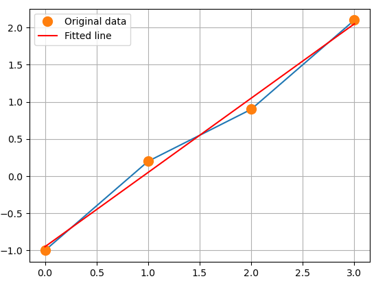
- 최소 제곱해를 선형 행렬 방정식으로 얻기
* linear_reg1.py
import numpy.linalg as lin
import numpy as np
import matplotlib.pyplot as plt
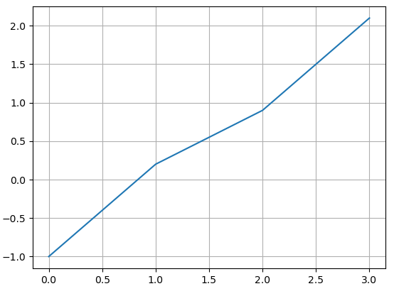
x = np.array([0, 1, 2, 3])
y = np.array([-1, 0.2, 0.9, 2.1])
plt.plot(x, y)
plt.grid(True)
plt.show()
A = np.vstack([x, np.ones(len(x))]).T
print(A)
'''
[[0. 1.]
 [1. 1.]
 [2. 1.]
 [3. 1.]]
'''

# y = mx + c
m, c = np.linalg.lstsq(A, y, rcond=None)[0]
print('기울기 :', m, ' y절편:', c) # 기울기 : 0.9999999999999997   y절편 : -0.949999999999999

plt.plot(x, y, 'o', label='Original data', markersize=10)
plt.plot(x, m*x + c, 'r', label='Fitted line')
plt.legend()
plt.show()
x = [8,3,6,6,9,4,3,9,3,4]
x = [800,300,600,600,900,400,300,900,300,400]
print('x 평균 :', np.mean(x)) # x 평균 : 5.5
print('x 분산 :', np.var(x))  # x 분산 : 5.45

y = [6,2,4,6,9,5,1,8,4,5]
y = [600,200,400,600,900,500,100,800,400,500]
print('y 평균 :', np.mean(y)) # y 평균 : 5.0
print('y 분산 :', np.var(y))  # y 분산 : 5.4
print()

# 두 변수 간의 관계확인
print('x, y 공분산 :', np.cov(x,y)[0, 1]) #  두 변수 간에 데이터 크기에 따라 동적
# x, y 공분산 : 5.222222222222222
print('x, y 상관계수 :', np.corrcoef(x, y)[0, 1]) # 두 변수 간에 데이터 크기에 따라 정적
# x, y 상관계수 : 0.8663686463212853

import matplotlib.pyplot as plt
plt.plot(x, y, 'o')
plt.show()
m = [-3, -2, -1, 0, 1, 2 , 3]
n = [9, 4, 1, 0, 1, 4, 9]

plt.plot(m, n, '+')
plt.show()
print('m, n 상관계수 :', np.corrcoef(m, n)[0, 1])
# m, n 상관계수 : 0.0
# 선형인 데이터만 사용 가능.
상관분석
: 두 변수 간에 상관관계의 강도를 분석 : 이론적 타당성(독립성) 확인. 독립변수 대상 변수들은 서로 간에 독립적이어야 함. : 독립변수 대상 변수들은 다중 공선성이 발생할 수 있는데, 이를 확인 : 밀도를 수치로 표현. 관계의 친밀함을 수치로 표현.
# heatmap : 밀도를 색으로 표현
import seaborn as sns
sns.heatmap(df.corr())
plt.show()
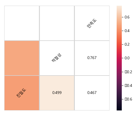
# hitmap에 텍스트 표시 추가사항 적용해 보기
corr = df.corr()
# Generate a mask for the upper triangle
mask = np.zeros_like(corr, dtype=np.bool)  # 상관계수값 표시
mask[np.triu_indices_from(mask)] = True
# Draw the heatmap with the mask and correct aspect ratio
vmax = np.abs(corr.values[~mask]).max()
fig, ax = plt.subplots()     # Set up the matplotlib figure

sns.heatmap(corr, mask=mask, vmin=-vmax, vmax=vmax, square=True, linecolor="lightgray", linewidths=1, ax=ax)

for i in range(len(corr)):
    ax.text(i + 0.5, len(corr) - (i + 0.5), corr.columns[i], ha="center", va="center", rotation=45)
    for j in range(i + 1, len(corr)):
        s = "{:.3f}".format(corr.values[i, j])
        ax.text(j + 0.5, len(corr) - (i + 0.5), s, ha="center", va="center")
ax.axis("off")
plt.show()
일원 카이제곱 : 변인 1 개 import scipy.stats as stats stats.chisquare()
일원 카이제곱 : 변인 2 개 이상 stats.chi2_contingency()
범주형
연속형
T 검정 : 범주형 값 2개 이하
단일 표본 검정 (one sample t-test) : 집단 1개 stats.ttest_1samp(데이터, popmean=모집단 평균)
독립 표본 검정(independent samples t test) : 두 집단 정규분포/ 분산 동일 stats.ttest_ind(데이터,..., , equal_var=False)
대응 표본 검정(paired samples t test) : 동일한 관찰 대상의 처리 전과 처리 후 비교 stats.ttest_rel(데이터, .. )
ANOVA :범주형 값 3개 이상
일원 분산분석(one-way anova) : 1개의 요인에 집단이 3개 import statsmodels.api as sm from statsmodels.formula.api import ols model = ols('종속변수 ~ 독립변수', data).fit() sm.stats.anova_lm(model, type=2)
model = ols('종속변수 ~ 독립변수1 + 독립변수2', data).fit()
stats.f_oneway(gr1, gr2, gr3)
연속형
범주형
로지스틱 회귀 분석
연속형
연속형
회귀분석, 구조 방정식
일원 분산분석(one-way anova)
: 1개의 요인에 집단이 3개
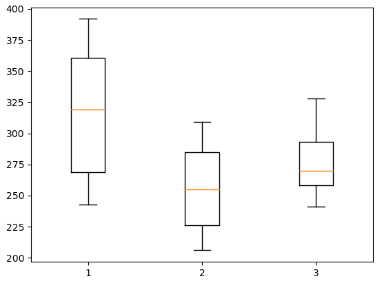
실습 1 : 세 가지 교육방법을 적용하여 1개월 동안 교육받은 교육생 80 명을 대상으로 실기시험을 실시 .
귀무가설 : 교육생을 대상으로 3가지 교육방법에 따른 실기시험 평균의 차이가 없다. 대립가설 : 교육생을 대상으로 3가지 교육방법에 따른 실기시험 평균의 차이가 있다.
* anova1.py
import pandas as pd
import scipy.stats as stats
import matplotlib.pyplot as plt

data = pd.read_csv('../testdata/three_sample.csv')
print(data.head(3), data.shape)
'''
   no  method  survey  score
0   1       1       1     72
1   2       3       1     87
2   3       2       1     78 (80, 4)
'''
print(data.describe())
- 이상치 제거
data = data.query('score <= 100')
plt.boxplot(data.score)
#plt.show()
귀무가설 : 태아와 관측자수는 태아의 머리둘레의 평균과 관련이 없다. 대립가설 : 태아와 관측자수는 태아의 머리둘레의 평균과 관련이 있다.
* anova.py
import scipy.stats as stats
import pandas as pd
import  numpy as np
import urllib.request
import matplotlib.pyplot as plt
plt.rc('font', family="malgun gothic")
from statsmodels.formula.api import ols
from statsmodels.stats.anova import anova_lm

url = "https://raw.githubusercontent.com/pykwon/python/master/testdata_utf8/group3_2.txt"
data = pd.read_csv(urllib.request.urlopen(url), delimiter=',')
print(data)
'''
    머리둘레  태아수  관측자수
0   14.3    1     1
1   14.0    1     1
2   14.8    1     1
3   13.6    1     2
4   13.6    1     2

'''

data.boxplot(column='머리둘레', by='태아수', grid=False)
plt.show()
reg = ols('data["머리둘레"] ~ C(data["태아수"]) + C(data["관측자수"])', data = data).fit()
result = anova_lm(reg, type=2)
print(result)
'''
                   df      sum_sq     mean_sq            F        PR(>F)
C(data["태아수"])    2.0  324.008889  162.004444  2023.182239  1.006291e-32
C(data["관측자수"])   3.0    1.198611    0.399537     4.989593  6.316641e-03
Residual         30.0    2.402222    0.080074          NaN           NaN
'''

# 두개의 요소 상호작용이 있는 형태로 처리
formula = '머리둘레 ~ C(태아수) + C(관측자수) + C(태아수):C(관측자수)'
reg2 = ols(formula, data).fit()
print(reg2)
result2 = anova_lm(reg2, type=2)
print(result2)
'''
                  df      sum_sq     mean_sq            F        PR(>F)
C(태아수)           2.0  324.008889  162.004444  2113.101449  1.051039e-27
C(관측자수)          3.0    1.198611    0.399537     5.211353  6.497055e-03
C(태아수):C(관측자수)   6.0    0.562222    0.093704     1.222222  3.295509e-01
Residual        24.0    1.840000    0.076667          NaN           NaN
'''
p-value PR(>F) C(태아수):C(관측자수) : 3.295509e-01 > 0.05 이므로 귀무가설 채택. # 귀무가설 : 태아와 관측자수는 태아의 머리둘레의 평균과 관련이 없다.
jikwon 테이블 정보로 chi, t검정, anova
* anova5_t.py
import MySQLdb
import ast
import pandas as pd
import numpy as np
import scipy.stats as stats
import statsmodels.stats.api as sm
import matplotlib.pyplot as plt

try:
    with open('mariadb.txt', 'r') as f:
        config = f.read()
except Exception as e:
    print('err :', e)

config = ast.literal_eval(config)

conn = MySQLdb.connect(**config)
cursor = conn.cursor()
print("=================================================================")
print(' * 교차분석 (이원 카이제곱 검정 : 각 부서(범주형)와 직원평가 점수(범주형) 간의 관련성 분석) *')
# 독립변수 : 범주형, 종속변수 : 범주형
# 귀무가설 : 각 부서와 직원평가 점수 간 관련이 없다.(독립)
# 대립가설 : 각 부서와 직원평가 점수 간 관련이 있다.

df = pd.read_sql("select * from jikwon", conn)
print(df.head(3))
'''
   jikwon_no jikwon_name  buser_num  ... jikwon_ibsail  jikwon_gen jikwon_rating
0          1         홍길동         10  ...    2008-09-01           남             a
1          2         한송이         20  ...    2010-01-03           여             b
2          3         이순신         20  ...    2010-03-03           남             b
'''

buser = df['buser_num']
rating = df['jikwon_rating']

ctab = pd.crosstab(buser, rating) # 교차표 작성
print(ctab)
'''
jikwon_rating  a  b  c
buser_num
10             5  1  1
20             3  6  3
30             5  2  0
40             2  2  0
'''

chi, p, df, exp = stats.chi2_contingency(ctab)
print('chi : {}, p : {}, df : {}'.format(chi, p, df))
# chi : 7.339285714285714, p : 0.2906064076671985, df : 6
# p-value : 0.2906 > 0.05 이므로 귀무가설 채택.
# 귀무가설 : 각 부서와 직원평가 점수 간 관련이 없다.(독립)
print("=================================================================")
print(' * 교차분석 (이원 카이제곱 검정 : 각 부서(범주형)와 직급(범주형) 간의 관련성 분석) *')
# 귀무가설 : 각 부서와 직급 간 관련이 없다.(독립)
# 대립가설 : 각 부서와 직급 간 관련이 있다.

df2 = pd.read_sql("select buser_num, jikwon_jik from jikwon", conn)
print(df2.head(3))
buser = df2.buser_num
jik = df2.jikwon_jik

ctab2 = pd.crosstab(buser, jik) # 교차표 작성
print(ctab2)

chi, p, df, exp = stats.chi2_contingency(ctab2)
print('chi : {}, p : {}, df : {}'.format(chi, p, df))
# chi : 9.620617477760335, p : 0.6492046290079438, df : 12
# p-value : 0.6492 > 0.05 이므로 귀무가설 채택.
# 귀무가설 : 각 부서와 직급 간 관련이 없다.(독립)
print()
print("=================================================================")
print(' * 차이분석 (t-test : 10, 20번 부서(범주형)와 평균 연봉(연속형) 간의 차이 분석) *')
# 독립변수 : 범주형, 종속변수 : 연속형

# 귀무가설 : 두 부서 간 연봉 평균의 차이가 없다.
# 대립가설 : 두 부서 간 연봉 평균의 차이가 있다.

#df_10 = pd.read_sql("select buser_num, jikwon_pay from jikwon where buser_num in (10, 20)", conn)
df_10 = pd.read_sql("select buser_num, jikwon_pay from jikwon where buser_num = 10", conn)
df_20 = pd.read_sql("select buser_num, jikwon_pay from jikwon where buser_num = 20", conn)
buser_10 = df_10['jikwon_pay']
buser_20 = df_20['jikwon_pay']

print('평균 :',np.mean(buser_10), ' ', np.mean(buser_20))
# 평균 : 5414.285714285715   4908.333333333333

t_result = stats.ttest_ind(buser_10, buser_20)
print(t_result)
# pvalue=0.6523 > 0.05 이므로 귀무가설 채택
# 귀무가설 : 두 부서 간 연봉 평균의 차이가 없다.
print()
print("=================================================================")
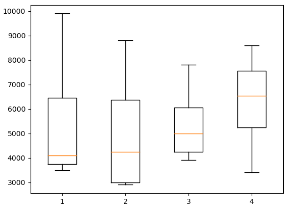
print(' * 분산분석 (ANOVA : 각 부서(부서라는 1개의 요인에 4그룹으로 분리. 범주형)와 평균 연봉(연속형) 간의 차이 분석) *')
# 독립변수 : 범주형, 종속변수 : 연속형
# 귀무가설 : 4개의 부서 간 연봉 평균의 차이가 없다.
# 대립가설 : 4개의 부서 간 연봉 평균의 차이가 있다.
df3 = pd.read_sql("select buser_num, jikwon_pay from jikwon", conn)
buser = df3['buser_num']
pay = df3['jikwon_pay']
gr1 = df3[df3['buser_num'] == 10 ]['jikwon_pay']
gr2 = df3[df3['buser_num'] == 20 ]['jikwon_pay']
gr3 = df3[df3['buser_num'] == 30 ]['jikwon_pay']
gr4 = df3[df3['buser_num'] == 40 ]['jikwon_pay']
print(gr1)
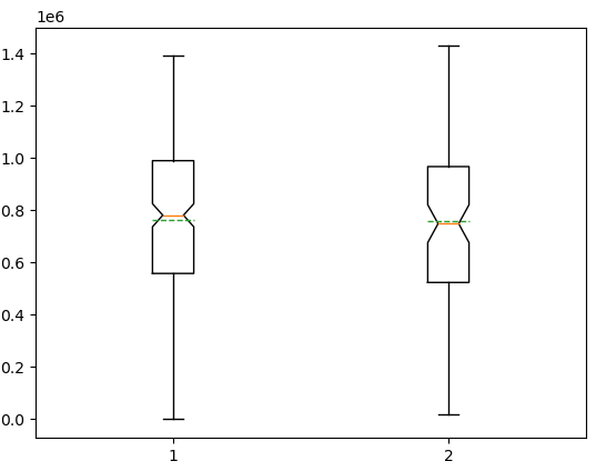
# 시각화
plt.boxplot([gr1, gr2, gr3, gr4])
#plt.show()
# 방법 1
f_sta, pv = stats.f_oneway(gr1, gr2, gr3, gr4)
print('f : {}, p : {}'.format(f_sta, pv))
# f : 0.41244077160708414, p : 0.7454421884076983
# p > 0.05 이므로 귀무가설 채택
# 귀무가설 : 4개의 부서 간 연봉 평균의 차이가 없다.
# 방법 2
lmodel = ols('jikwon_pay ~ C(buser_num)', data = df3).fit()
result = anova_lm(lmodel, type=2)
print(result)
'''
df sum_sq mean_sq F PR(>F)
C(buser_num) 3.0 5.642851e+06 1.880950e+06 0.412441 0.745442
Residual 26.0 1.185739e+08 4.560535e+06 NaN NaN
'''
# P : 0.745442 > 0.05 이므로 귀무가설 채택
# 귀무가설 : 4개의 부서 간 연봉 평균의 차이가 없다.
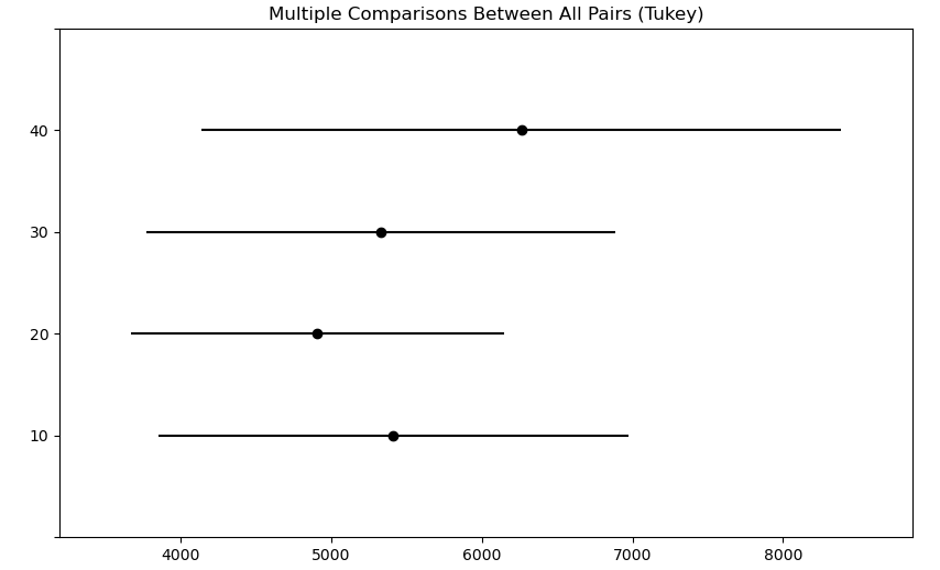
# 사후검정
from statsmodels.stats.multicomp import pairwise_tukeyhsd
tukey = pairwise_tukeyhsd(df3.jikwon_pay, df3.buser_num)
print(tukey)
'''
Multiple Comparison of Means - Tukey HSD, FWER=0.05
==========================================================
group1 group2 meandiff p-adj lower upper reject
----------------------------------------------------------
10 20 -505.9524 0.9 -3292.2958 2280.391 False
10 30 -85.7143 0.9 -3217.2939 3045.8654 False
10 40 848.2143 0.9 -2823.8884 4520.3169 False
20 30 420.2381 0.9 -2366.1053 3206.5815 False
20 40 1354.1667 0.6754 -2028.326 4736.6593 False
30 40 933.9286 0.8955 -2738.1741 4606.0312 False
'''
tukey.plot_simultaneous()
plt.show()
pvalue=0.02568 < 0.05 이므로 귀무가설 기각. # 대립가설 : 학생들의 국어점수의 평균은 80이 아니다.
실습4 : 여아 신생아 몸무게의 평균 검정 수행
여아 신생아의 몸무게는 평균이 2800(g) 으로 알려져 왔으나 이보다 더 크다는 주장이 나왔다. 표본으로 여아 18 명을 뽑아 체중을 측정하였다고 할 때 새로운 주장이 맞는지 검정해 보자
귀무가설 : 여아 신생아 몸무게의 평균이 2800g이다. 대립가설 : 여아 신생아 몸무게의 평균이 2800g 보다 크다.
data = pd.read_csv("https://raw.githubusercontent.com/pykwon/python/master/testdata_utf8/babyboom.csv")
print(data.head(3))
'''
   time  gender  weight  minutes
0     5       1    3837        5
1   104       1    3334       64
2   118       2    3554       78
'''
print(data.describe()) # gender - 1 : 여아, 2: 남아

fdata = data[data.gender == 1]
print(fdata.head(3), len(fdata), np.mean(fdata.weight))
'''
   time  gender  weight  minutes
0     5       1    3837        5
1   104       1    3334       64
5   405       1    2208      245
18명, 평균 : 3132.4444444444443
'''
# 3132(g)과 2800(g)에 대해 평균에 차이가 있는 지 검정.
# 정규성 확인
# 통계 추론시 대부분이 모집단은 정규분포를 따른다는 가정하에 진행하는 것이 일반적이다. 중심 극한의 원리에 의해
# 중심 극한의 원리 : 표본의 크기가 커질 수록 표본 평균의 분포는 모집단의 분포 모양과는 관계없이 정규 분포에 가까워진다.
print(stats.shapiro(fdata.weight)) # p-value=0.0179 < 0.05 => 정규성 위반
import matplotlib.pyplot as plt
import seaborn as sns
sns.distplot(fdata.iloc[:, 2], fit=stats.norm)
plt.show()
stats.probplot(fdata.iloc[:, 2], plot=plt) # Q-Q plot 상에서 정규성 확인 - 잔차의 정규성
plt.show()
stats.probplot(데이터, plot=plt) : Q-Q plot 상에서 정규성 확인 - 잔차의 정규성
import matplotlib.pyplot as plt
import seaborn as sns
sns.distplot(sco1, kde = False, fit=stats.norm)
sns.distplot(sco2, kde = False, fit=stats.norm)
plt.show()
결론 : pvalue=0.9195 > 0.05 이므로 귀무가설 채택. # 귀무가설 : 강수여부에 따른 매출액 평균에 차이가 없다.
서로 대응인 두 집단의 평균 차이 검정 (paired samples t test)
: 처리 이전과 처리 이후를 각각의 모집단으로 판단하여 동일한 관찰 대상으로부터 처리 이전과 처리 이후를 1:1 로 대응시킨 두 집단으로 부터의 표본을 대응표본 (paired sample) 이라고 한다. : 대응인 두 집단의 평균 비교는 동일한 관찰 대상으로부터 처리 이전의 관찰과 이후의 관찰을 비교하여 영향을 미친 정도를 밝히는데 주로 사용하고 있다 집단 간 비교가 아니므로 등분산 검정을 할 필요가 없다. : 광고 전/후의 상품 판매량의 차이, 운동 전/후의 근육량의 차이
실습 1 :특강 전/후의 시험점수는 차이
귀무가설 : 특강 전/후의 시험점수는 차이가 없다. 대립가설 : 특강 전/후의 시험점수는 차이가 있다.
* t5.py
import numpy as np
import scipy.stats as stats
from seaborn.distributions import distplot

# 대응 표본 t 검정 1
np.random.seed(12)
x1 = np.random.normal(80, 10, 100)
x2 = np.random.normal(77, 10, 100)
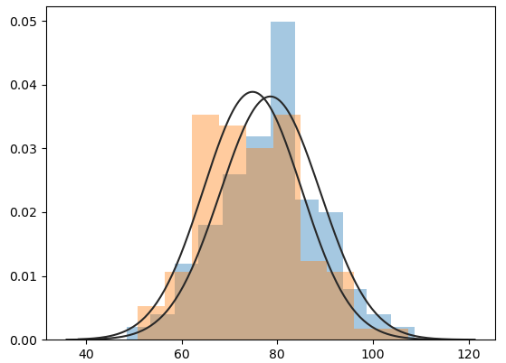
# 정규성
import matplotlib.pyplot as plt
import seaborn as sns
sns.distplot(x1, kde=False, fit=stats.norm)
sns.distplot(x2, kde=False, fit=stats.norm)
plt.show()
① 분포표 사용 -> 임계값 산출 임계값이 critical value 왼쪽에 있을 경우 귀무가설 채택/기각.
② p-value 사용(tool에서 산출). 유의확률. (경험적 수치) p-value > 0.05(a) : 귀무가설 채택. 우연히 발생할 확률이 0.05보다 낮아 연구가설 기각. p-value < 0.05(a) : 귀무가설 기각. 좋다 p-value < 0.01(a) : 귀무가설 기각. 더 좋다 p-value < 0.001(a) : 귀무가설 기각. 더 더 좋다 => 신뢰 할 수 있다.
척도에 따른 데이터 분석방법
독립변수 x
종속변수 y
분석 방법
범주형
범주형
카이제곱 검정(교차분석)
범주형
연속형
T 검정(범주형 값 2개 : 집단 2개 이하), ANOVA(범주형 값 3개 : 집단 2개 이상)
연속형
범주형
로지스틱 회귀 분석
연속형
연속형
회귀분석, 구조 방정식
1종 오류 : 귀무가설이 채택(참)인데, 이를 기각. 2종 오류 : 귀무가설이 기각(거짓)인데, 이를 채택.
분산(표준편차)의 중요도 - 데이터의 분포
* temp.py
import scipy.stats as stats
import numpy as np
import matplotlib.pyplot as plt

centers = [1, 1.5, 2] # 3개 집단
col = 'rgb'
data = []
std = 0.01 # 표준편차 - 작으면 작을 수록 응집도가 높다.

for i in range(len(centers)):
    data.append(stats.norm(centers[i], std).rvs(100)) # norm() : 가우시안 정규분포. rvs(100) : 랜덤값 생성.
    plt.plot(np.arange(100) + i * 100, data[i], color=col[i])   # 그래프
    plt.scatter(np.arange(100) + i * 100, data[i], color=col[i]) # 산포도
plt.show()
print(data)
import scipy.stats as stats
stats.norm(평균, 표준편차).rvs(size=크기, random_state=seed) : 가우시안 정규 분포 랜덤 값 생성.
import matplotlib.pyplot as plt
plt.plot(x, y) : 그래프 출력.
plot - std : 0.01
plot - std : 0.1scatter - std : 0.01
scatter - std : 0.1
교차분석 (카이제곱) 가설 검정
데이터나 집단의 분산을 추정하고 검정할때 사용
독립변수, 종속변수 : 범주형
일원 카이제곱 : 변수 단수. 적합성(선호도) 검정. 교차분할표 사용하지않음.
이원 카이제곱 : 변수 복수. 독립성(동질성) 검정. 교차분할표 사용.
절차 : 가설 설정 -> 유의 수준 결정 -> 검정통계량 계산 -> 귀무가설 채택여부 판단 -> 검정결과 진술
# 결론 : p-value 1.1679064204212775e-18 < 0.05 이므로 귀무가설 기각. ( 대립가설 : 연령대별로 SNS 서비스 이용 현황에 차이가 있다(동질이 없다) )
# 참고 : 상기 데이터가 모집단이었다면 샘플링을 진행하여 샘플링 데이터로 작업 진행.
sample_data = data2.sample(500, replace=True)
카이제곱 + Django
= django_use02_chi(PyDev Django Project)
Create application - coffesurvey
* settings
...

INSTALLED_APPS = [

    ...

    'coffeesurvey',
]

...

DATABASES = {
    'default': {
        'ENGINE': 'django.db.backends.mysql',
        'NAME': 'coffeedb',            # DB명 : db는 미리 작성되어 있어야 함.
        'USER': 'root',                # 계정명
        'PASSWORD': '123',             # 계정 암호
        'HOST': '127.0.0.1',           # DB가 설치된 컴의 ip
        'PORT': '3306',                # DBMS의 port 번호
    }
}
* MariaDB
create database coffeedb;

use coffeedb;

create table survey(rnum int primary key auto_increment, gender varchar(4),age int(3),co_survey varchar(10));

insert into survey (gender,age,co_survey) values ('남',10,'스타벅스');
insert into survey (gender,age,co_survey) values ('여',20,'스타벅스');
* anaconda prompt
cd C:\work\psou\django_use02_chi

python manage.py inspectdb > aaa.py
* models
from django.db import models

# Create your models here.
class Survey(models.Model):
    rnum = models.AutoField(primary_key=True)
    gender = models.CharField(max_length=4, blank=True, null=True)
    age = models.IntegerField(blank=True, null=True)
    co_survey = models.CharField(max_length=10, blank=True, null=True)

    class Meta:
        managed = False
        db_table = 'survey'
Make migrations - coffeesurvey
Migrate
* urls(django_use02_chi)
from django.contrib import admin
from django.urls import path
from coffeesurvey import views
from django.urls.conf import include

urlpatterns = [
    path('admin/', admin.site.urls),
    path('', views.Main), # url 없을 경우
    path('coffee/', include('coffeesurvey.urls')), # 위임
]
* views
from django.shortcuts import render
from coffeesurvey.models import Survey

# Create your views here.
def Main(request):
    return render(request, 'main.html')

...
# 인구통계 dataset 읽기
des = pd.read_csv('https://raw.githubusercontent.com/pykwon/python/master/testdata_utf8/descriptive.csv')
print(des.info())

# 5개 칼럼만 선택하여 data frame 생성
data = des[['resident','gender','age','level','pass']]
print(data[:5])

# 지역과 성별 칼럼 교차테이블
table = pd.crosstab(data.resident, data.gender)
print(table)

# 지역과 성별 칼럼 기준 - 학력수준 교차테이블
table = pd.crosstab([data.resident, data.gender], data.level)
print(table)
    # jikwon.csv 파일로 저장
    with open('jikwon.csv', 'w', encoding='utf-8') as fw:
        writer = csv.writer(fw)
        for row in cursor:
            writer.writerow(row)
        print('저장성공')
matplotlib : ploting library. 그래프 생성을 위한 다양한 함수 지원.
* mat1.py
import numpy as np
import matplotlib.pyplot as plt

plt.rc('font', family = 'malgun gothic')   # 한글 깨짐 방지
plt.rcParams['axes.unicode_minus'] = False # 음수 깨짐 방지

x = ["서울", "인천", "수원"]
y = [5, 3, 7]
# tuple 가능. set 불가능.

plt.xlabel("지역")                 # x축 라벨
plt.xlim([-1, 3])                 # x축 범위
plt.ylim([0, 10])                 # y축 범위
plt.yticks(list(range(0, 11, 3))) # y축 칸 number 지정
plt.plot(x, y)                    # 그래프 생성
plt.show()                        # 그래프 출력
data = np.arange(1, 11, 2)
print(data)    # [1 3 5 7 9]
plt.plot(data) # 그래프 생성
x = [0, 1, 2, 3, 4]
for a, b in zip(x, data):
    plt.text(a, b, str(b)) # 그래프 라인에 text 표시
plt.show()     # 그래프 출력
x = np.arange(10)
y = np.sin(x)
print(x, y)
plt.plot(x, y, 'bo')  # 파란색 o로 표시. style 옵션 적용.
plt.plot(x, y, 'r+')  # 빨간색 +로 표시
plt.plot(x, y, 'go--', linewidth = 2, markersize = 10) # 초록색 o 표시
plt.show()
# 홀드 : 그림 겹쳐 보기
x = np.arange(0, np.pi * 3, 0.1)
print(x)
y_sin = np.sin(x)
y_cos = np.cos(x)
plt.plot(x, y_sin, 'r')     # 직선, 곡선
plt.scatter(x, y_cos)       # 산포도
#plt.plot(x, y_cos, 'b')
plt.xlabel('x축')
plt.ylabel('y축')
plt.legend(['사인', '코사인']) # 범례
plt.title('차트 제목')         # 차트 제목
plt.show()
irum = ['a', 'b', 'c', 'd', 'e']
kor = [80, 50, 70, 70, 90]
eng = [60, 70, 80, 70, 60]
plt.plot(irum, kor, 'ro-')
plt.plot(irum, eng, 'gs--')
plt.ylim([0, 100])
plt.legend(['국어', '영어'], loc = 4)
plt.grid(True)          # grid 추가

fig = plt.gcf()         # 이미지 저장 선언
plt.show()              # 이미지 출력
fig.savefig('test.png') # 이미지 저장

from matplotlib.pyplot import imread
img = imread('test.png') # 이미지 read
plt.imshow(img)          # 이미지 출력
plt.show()
차트의 종류 결정
* mat2.py
import numpy as np
import matplotlib.pyplot as plt

fig = plt.figure()             # 명시적으로 차트 영역 객체 선언
ax1 = fig.add_subplot(1, 2, 1) # 1행 2열 중 1열에 표기
ax2 = fig.add_subplot(1, 2, 2) # 1행 2열 중 2열에 표기

ax1.hist(np.random.randn(10), bins=10, alpha=0.9) # 히스토그램 출력 - bins : 구간 수, alpha: 투명도
ax2.plot(np.random.randn(10)) # plot 출력
plt.show()
n = 30
np.random.seed(42)
x = np.random.rand(n)
y = np.random.rand(n)
color = np.random.rand(n)
scale = np.pi * (15 * np.random.rand(n)) ** 2
plt.scatter(x, y, s = scale, c = color)
plt.show()
import pandas as pd
sdata = pd.Series(np.random.rand(10).cumsum(), index = np.arange(0, 100, 10))
plt.plot(sdata)
plt.show()
import matplotlib.pyplot as plt
import seaborn as sns

titanic = sns.load_dataset("titanic")
print(titanic.info())
print(titanic.head(3))

age = titanic['age']
sns.kdeplot(age) # 밀도
plt.show()
sns.distplot(age) # kdeplot + hist
plt.show()
import matplotlib.pyplot as plt
import seaborn as sns
titanic = sns.load_dataset("titanic")
print(titanic.info())
print(titanic.head(3))
age = titanic['age']
sns.kdeplot(age) # 밀도
plt.show()
sns.relplot(x = 'who', y = 'age', data=titanic)
plt.show()
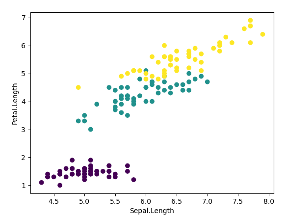
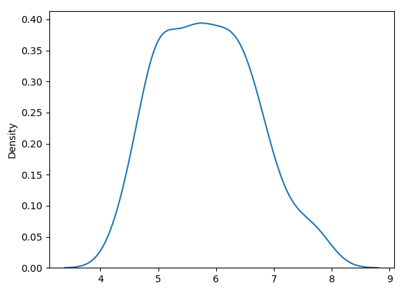
x = iris_data['Sepal.Length'].values
sns.rugplot(x)
plt.show()
sns.kdeplot(x)
plt.show()
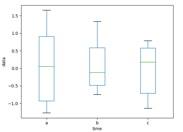
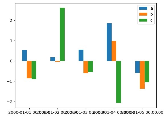
# pandas의 시각화 기능
import numpy as np
df = pd.DataFrame(np.random.randn(10, 3), index = pd.date_range('1/1/2000', periods=10), columns=['a', 'b', 'c'])
print(df)
#df.plot() # 꺽은선
#df.plot(kind= 'bar')
df.plot(kind= 'box')
plt.xlabel('time')
plt.ylabel('data')
plt.show()
df[:5].plot.bar(rot=0)
plt.show()
* mat4.py
import pandas as pd
tips = pd.read_csv('../testdata/tips.csv')
print(tips.info())
print(tips.head(3))
'''
total_bill tip sex smoker day time size
0 16.99 1.01 Female No Sun Dinner 2
1 10.34 1.66 Male No Sun Dinner 3
2 21.01 3.50 Male No Sun Dinner 3
'''
tips['gender'] = tips['sex'] # sex 칼럼을 gender 칼럼으로 변경
del tips['sex']
print(tips.head(3))
'''
total_bill tip smoker day time size gender
0 16.99 1.01 No Sun Dinner 2 Female
1 10.34 1.66 No Sun Dinner 3 Male
2 21.01 3.50 No Sun Dinner 3 Male
'''
# tip 비율 추가
tips['tip_pct'] = tips['tip'] / tips['total_bill']
print(tips.head(3))
'''
total_bill tip smoker day time size gender tip_pct
0 16.99 1.01 No Sun Dinner 2 Female 0.059447
1 10.34 1.66 No Sun Dinner 3 Male 0.160542
2 21.01 3.50 No Sun Dinner 3 Male 0.166587
'''
축약연산, 누락된 데이터 처리, Sql Query, 데이터 조작, 인덱싱, 시각화 .. 등 다양한 기능을 제공.
1. Series : 일련의 데이터를 기억할 수 있는 1차원 배열과 같은 자료 구조로 명시적인 색인을 갖는다.
* pdex1.py
Series(순서가 있는 자료형) : series 생성
from pandas import Series
import numpy as np
obj = Series([3, 7, -5, 4]) # int
obj = Series([3, 7, -5, '4']) # string - 전체가 string으로 변환
obj = Series([3, 7, -5, 4.5]) # float - 전체가 float으로 변환
obj = Series((3, 7, -5, 4)) # tuple - 순서가 있는 자료형 사용 가능
obj = Series({3, 7, -5, 4}) # set - 순서가 없어 error 발생
print(obj, type(obj))
'''
0 3
1 7
2 -5
3 4
dtype: int64 <class 'pandas.core.series.Series'>
'''
Series( , index = ) : 색인 지정
obj2 = Series([3, 7, -5, 4], index = ['a', 'b', 'c', 'd']) # index : 색인 지정
print(obj2)
'''
a 3
b 7
c -5
d 4
dtype: int64
'''
np.sum(obj2) = obj2.sum()
print(sum(obj2), np.sum(obj2), obj2.sum()) # pandas는 numpy 함수를 기본적으로 계승해서 사용.
'''
9 9 9
'''
obj.values : value를 list형으로 리턴
obj.index : index를 object형으로 리턴
print(obj2.values) # 값만 출력
print(obj2.index) # index만 출력
'''
[ 3 7 -5 4]
Index(['a', 'b', 'c', 'd'], dtype='object')
'''
슬라이싱
'''
a 3
b 7
c -5
d 4
'''
print(obj2['a'], obj2[['a']])
# 3 a 3
print(obj2[['a', 'b']])
'''
a 3
b 7
'''
print(obj2['a':'c'])
'''
a 3
b 7
c -5
'''
print(obj2[2]) # -5
print(obj2[1:4])
'''
b 7
c -5
d 4
'''
print(obj2[[2,1]])
'''
c -5
b 7
'''
print(obj2 > 0)
'''
a True
b True
c False
d True
'''
print('a' in obj2)
# True
DataFrame : 표 모양(2차원)의 자료 구조. Series가 여러개 합쳐진 형태. 각 칼럼마다 type이 다를 수 있다.
from pandas import DataFrame
df = DataFrame(obj3) # Series로 DataFrame 생성
print(df)
'''
상품가격
mouse 5000
keyboard 25000
monitor 55000
'''
data = {
'irum':['홍길동', '한국인', '신기해', '공기밥', '한가해'],
'juso':['역삼동', '신당동', '역삼동', '역삼동', '신사동'],
'nai':[23, 25, 33, 30, 35]
}
print(data, type(data))
'''
{'irum': ['홍길동', '한국인', '신기해', '공기밥', '한가해'],
'juso': ['역삼동', '신당동', '역삼동', '역삼동', '신사동'],
'nai': [23, 25, 33, 30, 35]}
<class 'dict'>
'''
frame = DataFrame(data) # dict로 DataFrame 생성
print(frame)
'''
irum juso nai
0 홍길동 역삼동 23
1 한국인 신당동 25
2 신기해 역삼동 33
3 공기밥 역삼동 30
4 한가해 신사동 35
'''
print(frame['irum']) # 칼럼을 dict 형식으로 접근
'''
0 홍길동
1 한국인
2 신기해
3 공기밥
4 한가해
'''
print(frame.irum, ' ', type(frame.irum)) # 칼럼을 속성 형식으로 접근
'''
0 홍길동
1 한국인
2 신기해
3 공기밥
4 한가해
Name: irum, dtype: object
<class 'pandas.core.series.Series'>
'''
print(DataFrame(data, columns=['juso', 'irum', 'nai'])) # 칼럼의 순서변경
'''
juso irum nai
0 역삼동 홍길동 23
1 신당동 한국인 25
2 역삼동 신기해 33
3 역삼동 공기밥 30
4 신사동 한가해 35
'''
print()
frame2 = DataFrame(data, columns=['juso', 'irum', 'nai', 'tel'], index = ['a', 'b', 'c', 'd', 'e'])
print(frame2)
'''
juso irum nai tel
a 역삼동 홍길동 23 NaN
b 신당동 한국인 25 NaN
c 역삼동 신기해 33 NaN
d 역삼동 공기밥 30 NaN
e 신사동 한가해 35 NaN
'''
frame2['tel'] = '111-1111' # tel 칼럼의 모든행에 적용
print(frame2)
'''
juso irum nai tel
a 역삼동 홍길동 23 111-1111
b 신당동 한국인 25 111-1111
c 역삼동 신기해 33 111-1111
d 역삼동 공기밥 30 111-1111
e 신사동 한가해 35 111-1111
'''
print()
val = Series(['222-2222', '333-2222', '444-2222'], index = ['b', 'c', 'e'])
frame2['tel'] = val
print(frame2)
'''
juso irum nai tel
a 역삼동 홍길동 23 NaN
b 신당동 한국인 25 222-2222
c 역삼동 신기해 33 333-2222
d 역삼동 공기밥 30 NaN
e 신사동 한가해 35 444-2222
'''
print()
print(frame2.T) # 행과 열 swap
'''
a b c d e
juso 역삼동 신당동 역삼동 역삼동 신사동
irum 홍길동 한국인 신기해 공기밥 한가해
nai 23 25 33 30 35
tel NaN 222-2222 333-2222 NaN 444-2222
'''
print(frame2.values)
'''
[['역삼동' '홍길동' 23 nan]
['신당동' '한국인' 25 '222-2222']
['역삼동' '신기해' 33 '333-2222']
['역삼동' '공기밥' 30 nan]
['신사동' '한가해' 35 '444-2222']]
'''
print(frame2.values[0, 1]) # 0행 1열. 홍길동
print(frame2.values[0:2]) # 0 ~ 1행
'''
[['역삼동' '홍길동' 23 nan]
['신당동' '한국인' 25 '222-2222']]
'''
행/열 삭제
#frame3 = frame2.drop('d') # index가 d인 행 삭제
frame3 = frame2.drop('d', axis=0) # index가 d인 행 삭제
print(frame3)
'''
juso irum nai tel
a 역삼동 홍길동 23 NaN
b 신당동 한국인 25 222-2222
c 역삼동 신기해 33 333-2222
e 신사동 한가해 35 444-2222
'''
frame3 = frame2.drop('tel', axis = 1) # index가 tel인 열 삭제
print(frame3)
'''
juso irum nai
a 역삼동 홍길동 23
b 신당동 한국인 25
c 역삼동 신기해 33
d 역삼동 공기밥 30
e 신사동 한가해 35
'''
정렬
print(frame2.sort_index(axis=0, ascending=False)) # 행 단위. 내림차순
'''
juso irum nai tel
e 신사동 한가해 35 444-2222
d 역삼동 공기밥 30 NaN
c 역삼동 신기해 33 333-2222
b 신당동 한국인 25 222-2222
a 역삼동 홍길동 23 NaN
'''
print(frame2.sort_index(axis=1, ascending=True)) # 열 단위. 오름차순
'''
irum juso nai tel
a 홍길동 역삼동 23 NaN
b 한국인 신당동 25 222-2222
c 신기해 역삼동 33 333-2222
d 공기밥 역삼동 30 NaN
e 한가해 신사동 35 444-2222
'''
print(frame2.rank(axis=0)) # 행 단위. 사전 순위로 칼럼 값 순서를 매김
'''
juso irum nai tel
a 4.0 5.0 1.0 NaN
b 1.0 4.0 2.0 1.0
c 4.0 2.0 4.0 2.0
d 4.0 1.0 3.0 NaN
e 2.0 3.0 5.0 3.0
'''
print(frame2['juso'].value_counts()) # 칼럼의 개수
'''
역삼동 3
신사동 1
신당동 1
'''
문자열 자르기
data = {
'juso':['강남구 역삼동', '중구 신당동', '강남구 대치동'],
'inwon':[22,23,24]
}
fr = DataFrame(data)
print(fr)
'''
juso inwon
0 강남구 역삼동 22
1 중구 신당동 23
2 강남구 대치동 24
'''
result1 = Series([x.split()[0] for x in fr.juso])
result2 = Series([x.split()[1] for x in fr.juso])
print(result1)
'''
0 강남구
1 중구
2 강남구
'''
print(result2)
'''
0 역삼동
1 신당동
2 대치동
'''
print(result1.value_counts())
'''
강남구 2
중구 1
'''
재 색인, NaN, bool처리, 슬라이싱 관련 메소드, 연산
* pdex2.py
Series 재 색인
data = Series([1,3,2], index = (1,4,2))
print(data)
'''
1 1
4 3
2 2
'''
data2 = data.reindex((1,2,4)) # 해당 index 순서로 정렬
print(data2)
'''
1 1
2 2
4 3
'''
재색인 시 값 채워 넣기
data3 = data2.reindex([0,1,2,3,4,5]) # 대응 값이 없는 인덱스는 NaN(결측값)이 됨.
print(data3)
'''
0 NaN
1 1.0
2 2.0
3 NaN
4 3.0
5 NaN
'''
data3 = data2.reindex([0,1,2,3,4,5], fill_value = 333) # 대응 값이 없는 인덱스는 fill_value으로 대입.
print(data3)
'''
0 333
1 1
2 2
3 333
4 3
5 333
'''
data3 = data2.reindex([0,1,2,3,4,5], method='ffill') # 대응 값이 없는 인덱스는 이전 index의 값으로 대입.
print(data3)
data3 = data2.reindex([0,1,2,3,4,5], method='pad') # 대응 값이 없는 인덱스는 이전 index의 값으로 대입.
print(data3)
'''
0 NaN
1 1.0
2 2.0
3 2.0
4 3.0
5 3.0
'''
data3 = data2.reindex([0,1,2,3,4,5], method='bfill') # 대응 값이 없는 인덱스는 다음 index의 값으로 대입.
print(data3)
data3 = data2.reindex([0,1,2,3,4,5], method='backfill') # 대응 값이 없는 인덱스는 다음 index의 값으로 대입.
print(data3)
'''
0 1.0
1 1.0
2 2.0
3 3.0
4 3.0
5 NaN
'''
bool 처리 / 슬라이싱
df = DataFrame(np.arange(12).reshape(4,3), index=['1월', '2월', '3월', '4월'], columns=['강남', '강북', '서초'])
print(df)
'''
강남 강북 서초
1월 0 1 2
2월 3 4 5
3월 6 7 8
4월 9 10 11
'''
print(df['강남'])
'''
1월 0
2월 3
3월 6
4월 9
'''
print(df['강남'] > 3 ) # True나 False 반환
'''
1월 False
2월 False
3월 True
4월 True
'''
print(df[df['강남'] > 3] ) # 강남이 3보다 큰 값 월의 값을 출력
'''
강남 강북 서초
3월 6 7 8
4월 9 10 11
'''
df[df < 3] = 0 # 3보다 작으면 0 대입
print(df)
'''
강남 강북 서초
1월 0 0 0
2월 3 4 5
3월 6 7 8
4월 9 10 11
'''
print(df.loc['3월', :]) # 복수 indexing. loc : 라벨 지원. iloc : 숫자 지원
print(df.loc['3월', ])
# 3월 행의 모든 값을 출력
'''
강남 6
강북 7
서초 8
'''
print(df.loc[:'2월']) # 2월행 이하의 모든 값 출력
'''
강남 강북 서초
1월 0 0 0
2월 3 4 5
'''
print(df.loc[:'2월',['서초']]) # 2월 이하 서초 열만 출력
'''
서초
1월 0
2월 5
'''
print(df.iloc[2]) # 2행의 모든 값 출력
print(df.iloc[2, :]) # 2행의 모든 값 출력
'''
강남 6
강북 7
서초 8
'''
print(df.iloc[:3]) # 3행 미만 행 모든 값 출력
'''
강남 강북 서초
1월 0 0 0
2월 3 4 5
3월 6 7 8
'''
print(df.iloc[:3, 2]) # 3행 미만 행 2열 미만 출력
'''
1월 0
2월 5
3월 8
'''
print(df.iloc[:3, 1:3]) # 3행 미만 행 1~2열 출력
'''
강북 서초
1월 0 0
2월 4 5
3월 7 8
'''
연산
s1 = Series([1,2,3], index = ['a', 'b', 'c'])
s2 = Series([4,5,6,7], index = ['a', 'b', 'd', 'c'])
print(s1)
'''
a 1
b 2
c 3
'''
print(s2)
'''
a 4
b 5
d 6
c 7
'''
print(s1 + s2) # 인덱스가 값은 경우만 연산, 불일치시 NaN
print(s1.add(s2))
'''
a 5.0
b 7.0
c 10.0
d NaN
'''
df1 = DataFrame(np.arange(9).reshape(3,3), columns=list('kbs'), index=['서울', '대전', '부산'])
print(df1)
'''
k b s
서울 0 1 2
대전 3 4 5
부산 6 7 8
'''
df2 = DataFrame(np.arange(12).reshape(4,3), columns=list('kbs'), index=['서울', '대전', '제주', '수원'])
print(df2)
'''
k b s
서울 0 1 2
대전 3 4 5
제주 6 7 8
수원 9 10 11
'''
print(df1 + df2) # 대응되는 index만 연산
print(df1.add(df2))
'''
k b s
대전 6.0 8.0 10.0
부산 NaN NaN NaN
서울 0.0 2.0 4.0
수원 NaN NaN NaN
제주 NaN NaN NaN
'''
print(df1.add(df2, fill_value = 0)) # 대응되지않는 값은 0으로 대입 후 연산
'''
k b s
대전 6.0 8.0 10.0
부산 6.0 7.0 8.0
서울 0.0 2.0 4.0
수원 9.0 10.0 11.0
제주 6.0 7.0 8.0
'''
seri = df1.iloc[0] # 0행만 추출
print(seri)
'''
k 0
b 1
s 2
'''
print(df1)
'''
k b s
서울 0 1 2
대전 3 4 5
부산 6 7 8
'''
print(df1 - seri)
'''
k b s
서울 0 0 0
대전 3 3 3
부산 6 6 6
'''
df1 = pd.DataFrame({'data1':range(7), 'key':['b', 'b', 'a', 'c', 'a', 'a', 'b']})
print(df1)
'''
data1 key
0 0 b
1 1 b
2 2 a
3 3 c
4 4 a
5 5 a
6 6 b
'''
df2 = pd.DataFrame({'key':['a', 'b', 'd'], 'data2':range(3)})
print(df2)
'''
key data2
0 a 0
1 b 1
2 d 2
'''
print()
print(pd.merge(df1, df2)) # inner join
print(pd.merge(df1, df2, on = 'key')) # inner join
print(pd.merge(df1, df2, on = 'key', how = 'inner')) # inner join
'''
data1 key data2
0 0 b 1
1 1 b 1
2 6 b 1
3 2 a 0
4 4 a 0
5 5 a 0
'''
print(pd.merge(df1, df2, on = 'key', how = 'outer')) # full outer join
'''
data1 key data2
0 0.0 b 1.0
1 1.0 b 1.0
2 6.0 b 1.0
3 2.0 a 0.0
4 4.0 a 0.0
5 5.0 a 0.0
6 3.0 c NaN
7 NaN d 2.0
'''
print(pd.merge(df1, df2, on = 'key', how = 'left')) # left outer join
'''
data1 key data2
0 0 b 1.0
1 1 b 1.0
2 2 a 0.0
3 3 c NaN
4 4 a 0.0
5 5 a 0.0
6 6 b 1.0
'''
print(pd.merge(df1, df2, on = 'key', how = 'right')) # right outer join
'''
data1 key data2
0 2.0 a 0
1 4.0 a 0
2 5.0 a 0
3 0.0 b 1
4 1.0 b 1
5 6.0 b 1
6 NaN d 2
'''
공통 칼럼명이 없는 경우
df3 = pd.DataFrame({'key2':['a','b','d'], 'data2':range(3)})
print(df3)
'''
key2 data2
0 a 0
1 b 1
2 d 2
'''
print(df1)
'''
data1 key
0 0 b
1 1 b
2 2 a
3 3 c
4 4 a
5 5 a
6 6 b
'''
print(pd.merge(df1, df3, left_on = 'key', right_on = 'key2'))
'''
data1 key key2 data2
0 0 b b 1
1 1 b b 1
2 6 b b 1
3 2 a a 0
4 4 a a 0
5 5 a a 0
'''
print()
print(pd.concat([df1, df3]))
print(pd.concat([df1, df3], axis = 0)) # 열 단위
'''
data1 key key2 data2
0 0.0 b NaN NaN
1 1.0 b NaN NaN
2 2.0 a NaN NaN
3 3.0 c NaN NaN
4 4.0 a NaN NaN
5 5.0 a NaN NaN
6 6.0 b NaN NaN
0 NaN NaN a 0.0
1 NaN NaN b 1.0
2 NaN NaN d 2.0
'''
print(pd.concat([df1, df3], axis = 1)) # 행 단위
'''
data1 key key2 data2
0 0 b a 0.0
1 1 b b 1.0
2 2 a d 2.0
3 3 c NaN NaN
4 4 a NaN NaN
5 5 a NaN NaN
6 6 b NaN NaN
'''
피벗 테이블: 데이터의 행렬을 재구성하여 그륩화 처리
data = {'city':['강남', '강북', '강남', '강북'],
'year':[2000, 2001, 2002, 2002],
'pop':[3.3, 2.5, 3.0, 2]
}
df = pd.DataFrame(data)
print(df)
'''
city year pop
0 강남 2000 3.3
1 강북 2001 2.5
2 강남 2002 3.0
3 강북 2002 2.0
'''
print(df.pivot('city', 'year', 'pop')) # city별, year별 pop의 평균
print(df.set_index(['city', 'year']).unstack()) # 기존의 행 인덱스를 제거하고 첫번째 열 인덱스 설정
'''
year 2000 2001 2002
city
강남 3.3 NaN 3.0
강북 NaN 2.5 2.0
'''
print(df.pivot('year', 'city', 'pop')) # year별 , city별 pop의 평균
'''
city 강남 강북
year
2000 3.3 NaN
2001 NaN 2.5
2002 3.0 2.0
'''
print(df['pop'].describe())
'''
count 4.000000
mean 2.700000
std 0.571548
min 2.000000
25% 2.375000
50% 2.750000
75% 3.075000
max 3.300000
'''
groupby
hap = df.groupby(['city'])
print(hap.sum()) # city별 합
print(df.groupby(['city']).sum()) # city별 합
'''
year pop
city
강남 4002 6.3
강북 4003 4.5
'''
print(df.groupby(['city', 'year']).sum()) # city, year 별 합
'''
pop
city year
강남 2000 3.3
2002 3.0
강북 2001 2.5
2002 2.0
'''
print(df.groupby(['city', 'year']).mean()) # city, year별 평균
'''
pop
city year
강남 2000 3.3
2002 3.0
강북 2001 2.5
2002 2.0
'''
pivot_table : pivot, groupby의 중간 성격
print(df)
'''
city year pop
0 강남 2000 3.3
1 강북 2001 2.5
2 강남 2002 3.0
3 강북 2002 2.0
'''
print(df.pivot_table(index=['city']))
print(df.pivot_table(index=['city'], aggfunc=np.mean)) # default : aggfunc=np.mean
'''
pop year
city
강남 3.15 2001.0
강북 2.25 2001.5
'''
print(df.pivot_table(index=['city', 'year'], aggfunc=[len, np.sum]))
'''
len sum
pop pop
city year
강남 2000 1.0 3.3
2002 1.0 3.0
강북 2001 1.0 2.5
2002 1.0 2.0
'''
print(df.pivot_table(values=['pop'], index = 'city')) # city별 합의 평균
print(df.pivot_table(values=['pop'], index = 'city', aggfunc=np.mean))
'''
pop
city
강남 3.15
강북 2.25
'''
print(df.pivot_table(values=['pop'], index = 'city', aggfunc=len))
'''
pop
city
강남 2.0
강북 2.0
'''
print(df.pivot_table(values=['pop'], index = ['year'], columns=['city']))
'''
pop
city 강남 강북
year
2000 3.3 NaN
2001 NaN 2.5
2002 3.0 2.0
'''
print(df.pivot_table(values=['pop'], index = ['year'], columns=['city'], margins=True))
'''
pop
city 강남 강북 All
year
2000 3.30 NaN 3.3
2001 NaN 2.50 2.5
2002 3.00 2.00 2.5
All 3.15 2.25 2.7
'''
print(df.pivot_table(values=['pop'], index = ['year'], columns=['city'], margins=True, fill_value=0))
'''
pop
city 강남 강북 All
year
2000 3.30 0.00 3.3
2001 0.00 2.50 2.5
2002 3.00 2.00 2.5
All 3.15 2.25 2.7
'''
file i/o
* pdex4_fileio.py
import pandas as pd
#local
df = pd.read_csv(r'../testdata/ex1.csv')
#web
df = pd.read_csv(r'https://raw.githubusercontent.com/pykwon/python/master/testdata_utf8/ex1.csv')
print(df, type(df))
'''
bunho irum kor eng
0 1 홍길동 90 90
1 2 신기해 95 80
2 3 한국인 100 85
3 4 박치기 67 54
4 5 마당쇠 55 100 <class 'pandas.core.frame.DataFrame'>
'''
df = pd.read_csv(r'../testdata/ex2.csv', header=None)
print(df, type(df))
'''
0 1 2 3 4
0 1 2 3 4 hello
1 5 6 7 8 world
2 9 10 11 12 foo <class 'pandas.core.frame.DataFrame'>
'''
df = pd.read_csv(r'../testdata/ex2.csv', names=['a', 'b', 'c', 'd', 'e'])
print(df, type(df))
'''
a b c d e
0 1 2 3 4 hello
1 5 6 7 8 world
2 9 10 11 12 foo <class 'pandas.core.frame.DataFrame'>
'''
df = pd.read_csv(r'../testdata/ex2.csv', names=['a', 'b', 'c', 'd', 'e'], index_col = 'e')
print(df, type(df))
'''
a b c d
e
hello 1 2 3 4
world 5 6 7 8
foo 9 10 11 12 <class 'pandas.core.frame.DataFrame'>
'''
df = pd.read_csv(r'../testdata/ex3.txt')
print(df, type(df))
'''
A B C
0 aaa -0.264438 -1.026059 -0.619500
1 bbb 0.927272 0.302904 -0.032399
2 ccc -0.264273 -0.386314 -0.217601
3 ddd -0.871858 -0.348382 1.100491 <class 'pandas.core.frame.DataFrame'>
'''
df = pd.read_csv(r'../testdata/ex3.txt', sep = '\s+', skiprows=[1, 3])
print(df, type(df))
'''
A B C
bbb 0.927272 0.302904 -0.032399
ddd -0.871858 -0.348382 1.100491 <class 'pandas.core.frame.DataFrame'>
'''
df = pd.read_fwf(r'../testdata/data_fwt.txt', encoding = 'utf8', widths=(10, 3, 5), names = ('date', 'name', 'price'))
print(df, type(df))
'''
date name price
0 2017-04-10 네이버 32000
1 2017-04-11 네이버 34000
2 2017-04-12 네이버 33000
3 2017-04-10 코리아 22000
4 2017-04-11 코리아 21000
5 2017-04-12 코리아 24000 <class 'pandas.core.frame.DataFrame'>
'''
print(df['date'])
'''
0 2017-04-10
1 2017-04-11
2 2017-04-12
3 2017-04-10
4 2017-04-11
5 2017-04-12
'''
import xml.etree.ElementTree as etree
# 일반적인 형태의 파일읽기
xml_f = open("pdex5.xml","r", encoding="utf-8").read()
print(xml_f,"\n",type(xml_f)) # <class str> 이므로 str관련 명령만 사용 가능
print()
root = etree.fromstring(xml_f)
print(root,'\n', type(root)) # <class xml.etree.ElementTree.Element> Element 관련 명령 사용가능
print(root.tag, len(root.tag)) # items 5
<?xml version="1.0" encoding="UTF-8"?>
<!-- xml문서 최상위 해당 라인이 추가되어야 한다. -->
<items>
<item>
<name id="ks1">홍길동</name>
<tel>111-1111</tel>
<exam kor="90" eng="80"/>
</item>
<item>
<name id="ks2">신길동</name>
<tel>111-2222</tel>
<exam kor="100" eng="50"/>
</item>
</items>
Beautifulsoup : XML, HTML문서의 일부 자료 추출
* pdex6_beautifulsoup.py
# Beautifulsoup : XML, HTML문서의 일부 자료 추출
# 라이브러리 설치 beautifulsoup4, request, lxml
# find(), select()
import requests
from bs4 import BeautifulSoup
def go():
base_url = "http://www.naver.com/index.html"
#storing all the information including headers in the variable source code
source_code = requests.get(base_url)
#sort source code and store only the plaintext
plain_text = source_code.text # 문자열
#print(plain_text)
#converting plain_text to Beautiful Soup object so the library can sort thru it
convert_data = BeautifulSoup(plain_text, 'lxml') # lxml의 HTML 해석기 사용
# 해석 라이브러리
# BeautifulSoup(markup, "html.parser")
# BeautifulSoup(markup, "lxml")
# BeautifulSoup(markup, ["lxml", "xml"])
# BeautifulSoup(markup, "xml")
# BeautifulSoup(markup, html5lib)
# find 함수
# find()
# find_next()
# find_all()
for link in convert_data.findAll('a'): # a tag search
href = link.get('href') # href 속성 get
#href = base_url + link.get('href') #Building a clickable url
print(href) #displaying href
go()
Beautifulsoup의 find(), select()
* pdex7_beautifulsoup.py
from bs4 import BeautifulSoup
html_page = """
<html><body>
<h1>제목태그</h1>
<p>웹문서 읽기</p>
<p>원하는 자료 선택</p>
</body></html>
"""
print(html_page, type(html_page)) # <class str>
soup = BeautifulSoup(html_page, 'html.parser') # BeautifulSoup 객체 생성
print(type(soup)) # bs4.BeautifulSoup BeautifulSoup이 제공하는 명령 사용 가능
print()
h1 = soup.html.body.h1
print('h1 :', h1.string) # h1 : 제목태그
p1 = soup.html.body.p # 최초의 p
print('p1 :', p1.string) # p1 : 웹문서 읽기
p2 = p1.next_sibling # </p>
p2 = p1.next_sibling.next_sibling
print('p2 :', p2.string) # p2 : 원하는 자료 선택
find() 사용
html_page2 = """
<html><body>
<h1 id='title'>제목태그</h1>
<p>웹문서 읽기</p>
<p id='my'>원하는 자료 선택</p>
</body></html>
"""
soup2 = BeautifulSoup(html_page2, 'html.parser')
print(soup2.p, ' ', soup2.p.string) # 직접 최초 tag 선택가능
# <p>웹문서 읽기</p> 웹문서 읽기
print(soup2.find('p').string) # find('태그명')
# 웹문서 읽기
print(soup2.find('p', id='my').string) # find('태그명', id='아이디명')
# 원하는 자료 선택
print(soup2.find_all('p')) # find_all('태그명')
# [<p>웹문서 읽기</p>, <p id="my">원하는 자료 선택</p>]
print(soup2.find(id='title').string) # find(id='아이디명')
# 제목태그
print(soup2.find(id='my').string)
# 원하는 자료 선택
import re
links2 = soup3.find_all(href=re.compile(r'^https://'))
print(links2) # [<a href="https://www.naver.com">naver</a>, <a href="https://www.daum.net">daum</a>]
for k in links2:
print(k.attrs['href'])
# https://www.naver.com
# https://www.daum.net
select() 사용(css의 selector)
html_page4 = """
<html><body>
<div id='hello'>
<a href="https://www.naver.com">naver</a><br/>
<a href="https://www.daum.net">daum</a><br/>
<ul class="world">
<li>안녕</li>
<li>반가워</li>
</ul>
</div>
<div id='hi'>
seconddiv
</div>
</body></html>
"""
soup4 = BeautifulSoup(html_page4, 'lxml')
aa = soup4.select_one('div#hello > a').string # select_one() : 하나만 선택
print("aa :", aa) # aa : naver
bb = soup4.select("div#hello ul.world > li") # > : 직계, 공백 : 자손, select() : 복수 선택. 객체리턴.
print("bb :", bb) # bb : [<li>안녕</li>, <li>반가워</li>]
for i in bb:
print("li :", i.string)
# li : 안녕
# li : 반가워
웹문서 읽기 - web scraping
* pdex8.py
import urllib.request as req
from bs4 import BeautifulSoup
url = "https://ko.wikipedia.org/wiki/%EC%9D%B4%EC%88%9C%EC%8B%A0"
wiki = req.urlopen(url)
print(wiki) # <http.client.HTTPResponse object at 0x00000267F71B1550>
soup = BeautifulSoup(wiki, 'html.parser')
# Chrome - F12 - 태그 오른쪽 클릭 - Copy - Copy selector
print(soup.select_one("#mw-content-text > div.mw-parser-output > p"))
url = "https://news.daum.net/society#1"
daum = req.urlopen(url)
soup = BeautifulSoup(daum, 'html.parser')
print(soup.select_one("div#kakaoIndex > a").string) # 본문 바로가기
datas = soup.select("div#kakaoIndex > a")
for i in datas:
href = i.attrs['href']
text = i.string
print("href :{}, text:{}".format(href, text))
#print("href :%s, text:%s"%(href, text))
# href :#kakaoBody, text:본문 바로가기
# href :#kakaoGnb, text:메뉴 바로가기
print()
datas2 = soup.findAll('a')
#print(datas2)
for i in datas2[:2]:
href = i.attrs['href']
text = i.string
print("href :{}, text:{}".format(href, text))
# href :#kakaoBody, text:본문 바로가기
# href :#kakaoGnb, text:메뉴 바로가기
날씨 정보 예보
* pdex9_weather.py
#<![CDATA[ ]]>
import urllib.request
import urllib.parse
from bs4 import BeautifulSoup
import pandas as pd
url = "http://www.weather.go.kr/weather/forecast/mid-term-rss3.jsp"
data = urllib.request.urlopen(url).read()
#print(data.decode('utf-8'))
soup = BeautifulSoup(urllib.request.urlopen(url).read(), 'lxml')
#print(soup)
print()
title = soup.find('title').string
print(title) # 기상청 육상 중기예보
#wf = soup.find('wf')
wf = soup.select_one('item > description > header > wf')
print(wf)
city = soup.find_all('city')
#print(city)
cityDatas = []
for c in city:
#print(c.string)
cityDatas.append(c.string)
df = pd.DataFrame()
df['city'] = cityDatas
print(df.head(3))
'''
city
0 서울
1 인천
2 수원
'''
#tmEfs = soup.select_one('location data tmef')
#tmEfs = soup.select_one('location > data > tmef')
tmEfs = soup.select_one('location > province + city + data > tmef') # + 아래 형제
print(tmEfs) # <tmef>2021-02-28 00:00</tmef>
tempMins = soup.select('location > province + city + data > tmn')
tempDatas = []
for t in tempMins:
tempDatas.append(t.string)
df['temp_min'] = tempDatas
print(df.head(3), len(df))
'''
city temp_min
0 서울 3
1 인천 3
2 수원 2 41
'''
df.columns = ['지역', '최저기온']
print(df.head(3))
'''
지역 최저기온
0 서울 3
1 인천 3
2 수원 2
'''
print(df.describe())
print(df.info())
# 파일로 저장
df.to_csv('날씨정보.csv', index=False)
df2 = pd.read_csv('날씨정보.csv')
print(df2.head(2))
print(df2[0:2])
print(df2.tail(2))
print(df2[-2:len(df)])
'''
지역 최저기온
39 제주 10
40 서귀포 10
'''
print(df.iloc[0])
'''
지역 서울
최저기온 3
'''
print(type(df.iloc[0])) # Series
print(df.iloc[0:2, :])
'''
지역 최저기온
0 서울 3
1 인천 3
'''
print(type(df.iloc[0:2, :])) # DataFrame
print("---")
print(df.iloc[0:2, 0:2])
'''
지역 최저기온
0 서울 3
1 인천 3
0 서울
1 인천
'''
print(df['지역'][0:2])
'''
0 서울
1 인천
'''
print(df['지역'][:2])
'''
0 서울
1 인천
'''
print("---")
print(df.loc[1:3])
'''
지역 최저기온
1 인천 3
2 수원 2
3 파주 -2
'''
print(df.loc[[1, 3]])
'''
지역 최저기온
1 인천 3
3 파주 -2
'''
print(df.loc[:, '지역'])
'''
0 서울
1 인천
2 수원
3 파주
'''
print('----------')
df = df.astype({'최저기온':'int'})
print(df.info())
print('----------')
print(df['최저기온'].mean()) # 2.1951219512195124
print(df['최저기온'].std()) # 3.034958914014504
print(df['최저기온'].describe())
#print(df['최저기온'] >= 5)
print(df.loc[df['최저기온'] >= 5])
'''
지역 최저기온
17 여수 5
19 광양 5
27 부산 7
28 울산 5
32 통영 6
35 포항 6
39 제주 10
40 서귀포 10
'''
print('----------')
print(df.sort_values(['최저기온'], ascending=True))
'''
지역 최저기온
31 거창 -3
6 춘천 -3
3 파주 -2
4 이천 -2
34 안동 -2
13 충주 -1
7 원주 -1
'''
웹 문서를 다운받아 파일로 저장하기 - 스케줄러
* pdex10_schedule.py
# 웹 문서를 다운받아 파일로 저장하기 - 스케줄러
from bs4 import BeautifulSoup
import urllib.request as req
import datetime
def working():
url = "https://finance.naver.com/marketindex/"
data = req.urlopen(url)
soup = BeautifulSoup(data, 'html.parser')
price = soup.select_one("div.head_info > span.value").string
print("미국 USD :", price) # 미국 USD : 1,108.90
t = datetime.datetime.now()
print(t) # 2021-02-25 14:52:30.108522
fname = './usd/' + t.strftime('%Y-%m-%d-%H-%M-%S') + ".txt"
print(fname) # 2021-02-25-14-53-59.txt
with open(fname, 'w') as f:
f.write(price)
# 스케줄러
import schedule # pip install schedule
import time
# 한번만 실행
working();
# 10초에 한번씩 실행
schedule.every(10).second.do(working)
# 10분에 한번씩 실행
schedule.every(10).minutes.do(working)
# 매 시간 실행
schedule.every().hour.do(working)
# 매일 10:30 에 실행
schedule.every().day.at("10:30").do(working)
# 매주 월요일 실행
schedule.every().monday.do(working)
# 매주 수요일 13:15 에 실행
schedule.every().wednesday.at("13:15").do(working)
while True:
schedule.run_pending()
time.sleep(1)
urllib.request, requests 모듈로 웹 자료 읽기
* pdex11.py
방법 1
from bs4 import BeautifulSoup
import urllib.request
url = "https://movie.naver.com/movie/sdb/rank/rmovie.nhn" # 네이버 영화 랭킹 정보
data = urllib.request.urlopen(url).read()
print(data)
soup = BeautifulSoup(data, 'lxml')
print(soup)
print(soup.select("div.tit3"))
print(soup.select("div[class=tit3]")) # 위와 동일
for tag in soup.select("div[class=tit3]"):
print(tag.text.strip())
'''
미션 파서블
극장판 귀멸의 칼날: 무한열차편
소울
퍼펙트 케어
새해전야
몬스터 헌터
'''
방법 2
import requests
data = requests.get(url);
print(data.status_code, data.encoding) # 정보 반환. 200 MS949
datas = data.text
print(datas)
datas = requests.get(url).text; # 명령을 연속적으로 주고 읽음
soup2 = BeautifulSoup(datas, "lxml")
print(soup2)
m_list = soup2.findAll("div", "tit3") # findAll("태그명", "속성명")
m_list = soup2.findAll("div", {'class':'tit3'}) # findAll("태그명", {'속성':'속성명'})
print(m_list)
count = 1
for i in m_list:
title = i.find('a')
#print(title)
print(str(count) + "위 : " + title.string)
count += 1
'''
1위 : 미션 파서블
2위 : 극장판 귀멸의 칼날: 무한열차편
3위 : 소울
4위 : 퍼펙트 케어
5위 : 새해전야
6위 : 몬스터 헌터
7위 : 더블패티
'''
네이버 실시간 검색어
import requests
from bs4 import BeautifulSoup # html 분석 라이브러리
# 유저 설정
url = 'https://datalab.naver.com/keyword/realtimeList.naver?where=main'
headers = {'User-Agent':'Mozilla/5.0 (Windows NT 10.0; Win64; x64) AppleWebKit/537.36 (KHTML, like Gecko) Chrome/80.0.3987.122 Safari/537.36'}
res = requests.get(url, headers = headers)
soup = BeautifulSoup(res.content, 'html.parser')
# span.item_title 정보를 선택
data = soup.select('span.item_title')
i = 1
for item in data:
print(str(i) + ')' + item.get_text())
i += 1
'''
1)함소원 진화
2)함소원
3)오은영
4)기성용
'''
# XML로 제공된 강남구 도서간 정보 읽기
import urllib.request as req
from bs4 import BeautifulSoup
url = "http://openapi.seoul.go.kr:8088/sample/xml/SeoulLibraryTime/1/5/"
plainText = req.urlopen(url).read().decode() # url의 text read
#print(plainText)
xmlObj = BeautifulSoup(plainText, 'lxml') # xml 해석기 사용
libData = xmlObj.select('row') # row 태그의 데이터 정보 객체에 저장
#print(libData)
for data in libData:
name = data.find('lbrry_name').text # row태그내 lbrry_name 태그 정보 read
addr = data.find('adres').text # row태그내 adres 태그 정보 read
print('도서관명\t:', name,'\n주소\t:',addr)
import json
json_file = "./pdex14.json" # 파일경로
json_data = {}
def readData(filename):
f = open(filename, 'r', encoding="utf-8") # 파일 열기
lines = f.read() # 파일 읽기
f.close() # 파일 닫기
#print(lines)
return json.loads(lines) # decoding str -> dict
def main():
global json_file # 전역 변수 사용
json_data = readData(json_file) # json파일의 내용을 dict타입으로 반환
print(type(json_data)) # dict
d1 = json_data['직원']['이름'] # data의 key로 value read
d2 = json_data['직원']['직급']
d3 = json_data['직원']['전화']
print("이름 : " + d1 +" 직급 : "+d2 + " 전화 : "+d3)
# 이름 : 홍길동 직급 : 대리 전화 : 010-222-2222
if __name__ == "__main__":
main()
* pdex15_json.py
jsonData.get('태그명')
# JSON으로 제공된 강남구 도서간 정보 읽기
import urllib.request as req
import json
url = "http://openapi.seoul.go.kr:8088/sample/json/SeoulLibraryTime/1/5/ "
plainText = req.urlopen(url).read().decode() # url text read 및 decode
print(plainText)
jsonData = json.loads(plainText)
print(jsonData['SeoulLibraryTime']['row'][0]["LBRRY_NAME"]) # LH강남3단지작은도서관
# get 함수
libData = jsonData.get("SeoulLibraryTime").get("row")
print(libData)
name = libData[0].get('LBRRY_NAME') # LH강남3단지작은도서관
print(name)
print()
for msg in libData:
name = msg.get('LBRRY_NAME')
tel = msg.get('TEL_NO')
addr = msg.get('ADRES')
print('도서관명\t:', name,'\n주소\t:',addr,'\n전화\t:',tel)
'''
도서관명 : LH강남3단지작은도서관
주소 : 서울특별시 강남구 자곡로3길 22
전화 : 02-459-8700
도서관명 : 강남구립못골도서관
주소 : 서울시 강남구 자곡로 116
전화 : 02-459-5522
도서관명 : 강남역삼푸른솔도서관
주소 : 서울특별시 강남구 테헤란로8길 36. 4층
전화 : 02-2051-1178
도서관명 : 강남한신휴플러스8단지작은도서관
주소 : 서울특별시 강남구 밤고개로27길 20(율현동, 강남한신휴플러스8단지)
전화 :
도서관명 : 강남한양수자인작은씨앗도서관
주소 : 서울특별시 강남구 자곡로 260
전화 :
'''
selenium : 자동 웹 브라우저 제어
anaconda 접속
pip install selenium
https://sites.google.com/a/chromium.org/chromedriver/home 접속
Latest stable release: ChromeDriver 88.0.4324.96 접속
chromedriver_win32.zip download
dowload 파일 특정경로에 압축풀어 이동
anaconda 접속
python
from selenium import webdriver
browser = webdriver.Chrome('D:/1. 프로그래밍/0. 설치 Program/Python/chromedriver')
browser.implicitly_wait(5)
browser.get('https://daum.net')
browser.quit()
import time
from selenium import webdriver
browser = webdriver.Chrome('D:/1. 프로그래밍/0. 설치 Program/Python/chromedriver')
browser.get('http://www.google.com/xhtml');
time.sleep(5)
search_box = browser.find_element_by_name('q')
search_box.send_keys('파이썬')
search_box.submit()
time.sleep(5)
browser.quit()
* pdex16_selenium.py
# 셀레니움으로 임의의 사이트 화면 캡처
from selenium import webdriver
try:
url = "http://www.daum.net"
browser = webdriver.Chrome('D:/1. 프로그래밍/0. 설치 Program/Python/chromedriver')
browser.implicitly_wait(3)
browser.get(url);
browser.save_screenshot("daum_img.png")
browser.quit()
print('성공')
except Exception:
print('에러')
형태소 분석
* nlp01.py
# 말뭉치 : 자연어 연구를 목적으로 수집된 샘플 dataset
# 형태소(단어로써 의미를 가지는 최소 단위) 분석 (한글) - 어근, 접두사, 접미사, 품사 형태로 분리한 데이터로 분석작업
from konlpy.tag import Kkma
kkma = Kkma()
#print(kkma)
phrase = "영국 제약사 아스트라제네카의 백신 1차분 접종은 오전 9시부터 전국의 요양원 직원들과 약 5200만명의 환자들에게 투여되기 시작했다. 반가워요"
print(kkma.sentences(phrase))
print(kkma.nouns(phrase)) # 명사 출력
print()
from konlpy.tag import Okt
okt = Okt()
print(okt.pos(phrase)) # 단어 + 품사
print(okt.pos(phrase, stem=True)) #
print(okt.nouns(phrase)) # 명사 출력
print(okt.morphs(phrase)) # 모든 품사 출력
단어 빈도수
* nlp2_webscrap
# 위키백과 사이트에서 원하는 단어 검색 후 형태소 분석. 단어 출현 빈도 수 출력.
import urllib
from bs4 import BeautifulSoup
from konlpy.tag import Okt
from urllib import parse # 한글 인코딩용
okt = Okt()
#para = input('검색 단어 입력 : ')
para = "이순신"
para = parse.quote(para) # 한글 인코딩
url = "https://ko.wikipedia.org/wiki/" + para
print(url) # https://ko.wikipedia.org/wiki/%EC%9D%B4%EC%88%9C%EC%8B%A0
page = urllib.request.urlopen(url) # url 열기
#print(page)
soup = BeautifulSoup(page.read(), 'lxml') # url 읽어. xml 해석기 사용
#print(soup)
wordList = [] # 형태소 분석으로 명사만 추출해 기억
for item in soup.select("#mw-content-text > div > p"): # p태그의 데이터를 읽는다
#print(item)
if item.string != None: # 태그 내부가 비어있으면 저장 하지않는다.
#print(item.string)
ss = item.string
wordList += okt.nouns(ss) # 명사만 추출
print("wordList :", wordList)
print("단어 수 :", len(wordList))
'''
wordList : ['당시', '조산', '만호', '이순신', ...]
단어 수 : 241
'''
# 단어의 발생횟수를 dict type 당시 : 2 조산:5
word_dict = {}
for i in wordList:
if i in word_dict: # dict에 없으면 추가 있으면 count+1
word_dict[i] += 1
else:
word_dict[i] = 1
print("word_dict :", word_dict)
'''
word_dict : {'당시': 3, '조산': 1, '만호': 1, ...}
'''
setdata = set(wordList)
print(setdata)
print("단어 수(중복 제거 후) :", len(setdata)) # 단어 수(중복 제거 후) : 169
print()
# 판다스의 series type으로 처리
import pandas as pd
woList = pd.Series(wordList)
print(woList[:5])
print(woList.value_counts()[:5]) # 단어 별 횟수 총 갯수 top 5
'''
0 당시
1 조산
2 만호
3 이순신
4 북방
dtype: object
이순신 14
척 7
배 7
대한 5
그 4
dtype: int64
당시 3
조산 1
만호 1
이순신 14
북방 1
'''
print()
woDict = pd.Series(word_dict)
print(woDict[:5])
print(woDict.value_counts())
'''
1 133
2 23
3 7
7 2
4 2
14 1
5 1
'''
print()
# DataFrame으로 처리
df1 = pd.DataFrame(wordList, columns =['단어'])
print(df1.head(5))
print()
'''
단어
0 당시
1 조산
2 만호
3 이순신
4 북방
'''
# 단어 / 빈도수
df2 = pd.DataFrame([word_dict.keys(), word_dict.values()])
df2 = df2.T
df2.columns = ['단어', '빈도수']
print(df2.head(3))
'''
단어 빈도수
0 당시 3
1 조산 1
2 만호 1
'''
df2.to_csv("./이순신.csv", sep=',', index=False)
df3 = pd.read_csv("./이순신.csv")
print(df3.head(3))
'''
단어 빈도수
0 당시 3
1 조산 1
2 만호 1
'''
# 웹 뉴스 정보를 읽어 형태소 분석 = > 단어별 유사도 출력
import pandas as pd
from konlpy.tag import Okt
okt = Okt()
with open('news.txt', mode='r', encoding='utf8') as f:
#print(f.read())
lines = f.read().split('\n') # 줄 나누기
print(len(lines))
wordDic = {} # 단어 수 확인을 위한 dict type
for line in lines:
datas = okt.pos(line) # 품사 태깅
#print(datas) # [('(', 'Punctuation'), ('경남', 'Noun'), ('=', 'Punctuation'), ...
for word in datas:
if word[1] == 'Noun': # 명사만 작업에 참여
#print(word) # ('경남', 'Noun')
#print(word[0] in wordDic)
if not (word[0] in wordDic): # 없으면 0, 있으면 count + 1
wordDic[word[0]] = 0 # {word[0] : count, ... }
wordDic[word[0]] += 1
print(wordDic)
# {'경남': 9, '뉴스': 4, '김다솜': 1, '기자': 1, '가덕도': 14, ...
# 단어 건수 별 내림차순 정렬
keys = sorted(wordDic.items(), key= lambda x : x[1], reverse=True) # count로 내림차순 정렬
print(keys)
# DataFrame에 담기 - 단어, 건수
wordList = []
countList = []
for word, count in keys[:20]: #상위 20개만 작업
wordList.append(word)
countList.append(count)
df = pd.DataFrame()
df['word'] = wordList
df['count'] = countList
print(df)
'''
word count
0 공항 19
1 가덕도 14
2 경남 9
3 특별법 9
4 시민사회단체 8
5 도내 6
'''
# word2vec
result = []
with open('news.txt', mode='r', encoding='utf8') as fr:
lines = fr.read().split('\n') # 줄 나누기
for line in lines:
datas = okt.pos(line, stem=True) # 품사 태깅. stem : 원형 어근 형태로 처리. 한가하고 -> 한가하다
#print(datas) # [('(', 'Punctuation'), ('경남', 'Noun'), ('=', 'Punctuation'), ...
temp = []
for word in datas:
if not word[1] in ['Punctuation', 'Suffix', 'Josa', 'Verb', 'Modifier', 'Number', 'Determiner', 'Foreign']:
temp.append(word[0]) # 한 줄당 단어
temp2 = (" ".join(temp)).strip() # 공백 제거 후 띄어쓰기를 채워 합친다.
result.append(temp2)
print(result)
fileName = "news2.txt"
with open(fileName, mode="w", encoding='utf8') as fw:
fw.write('\n'.join(result)) # 각 줄을 \n로 이어준 후 저장
print('저장 완료')
경남 뉴스 김다솜 기자 가덕도 공항 특별법 국회통과 경남 도내 시민사회단체 정당 반대 의견 있다
경남 기후 위기 비상 행동 민주 노총 경남 본부 등 도내 시민사회단체 날 오전 경남 도청 앞 기자회견 관련 부처 반대 의견 표명 가덕도 공항 특별법 기득권 당 담합 행위 반발
정의당 남도 같다 입장 성명 발표
이 관련 부처 반대 사업 수 없다 강조 국토교통부 가덕도 공항 의견 보고서 위험성 효율 등 부정 측면 지적 만큼 신중하다 판단 것
국토교통부 지난 안정 공성 운영 등 가지 점검 내용 의견 보고서 제시 보고서 가덕도 공항 건설 시 안전 사고 위험성 크게 증가 환경 훼손 지적 있다
법무부 가덕도 공항 특별법 개별 구체 사건 규율 있다 적법 절차 및 평등 원칙 위배 우려 있다 입장 전
이번 가덕도 공항 특별법 포함 예비 타당성 조사 면제 대한 반응 좋다 기획재정부 대규모 신규 사업 예산 낭비 방지 타당성 검증 필요 있다 의견 전
도내 시민사회단체 관계 부처 수용 곤란하다 말 있다 며 설계 없이 공사 수 있다 유례 수 없다 이 기상 외한 가덕도 공항 특별법 위험하다 짝 없다 고 비판
가덕도 공항 특별법 처리 도내 시민사회단체 민주 노총 경남 본부 정의당 남도 법안 폐기 촉구 이 가덕도 공항 건설 피해 막대 점 거듭 강조 경남 시민사회단체 제공 뉴스
가덕도 공항 특별법 처리 도내 시민사회단체 민주 노총 경남 본부 정의당 남도 법안 폐기 촉구 이 가덕도 공항 건설 피해 막대 점 거듭 강조 경남 시민사회단체 제공 뉴스
당초 동남권 관문 공항 위 목적 지적도 부산시 발표 가덕도 공항 건설 국제선 개항 국내선 김해 공항 개항 동남권 관문 공항 보기 현실 못 설명
국제선 국내선 군시설 등 동남권 관문 공항 기본 요소 부산시 추산 원보 많다 원 필요하다 점도 이명박 정부 시행 대강 사업 예산 많다 액수
도내 시민사회단체 정부 여당 적폐 비난 이명박 대강 사업 더 며 동네 하천 정비 이렇게 고 일
정의당 남도 모든 분야 부 적격하다 가덕도 공항 특별법 건 집권 여당 명백하다 입법권 남용 라며 임시 부산시 자리 위해 백년 지대 공항 건설 선거 지대 전락 민주당 국민 힘 규탄 고 전
한편 가덕도 공항 특별법 오늘 국회 본회의 통과 전망 이 법안 예비 타당성조사 면제 다른 법률 우선 적용 내용 등 있다
allcotton@news1.kr
Copyright 뉴스 코리아 www.news1.kr 무단 복제 및 재 재 배포 금지
# 모델 생성
model = word2vec.Word2Vec(genObj, size=100, window=10, min_count=2, sg=1) # window : 참조 주변 단어 수, min_count : 2보다 적은 값은 모델 구성에서 제외, sg=0 cbow, sg=1 skip-gram,
#Cbow 주변 단어로 중심단어 예측
#skip-gram : 중심 단어로 주변단어 추측
print(model)
model.init_sims(replace=True) # 모델 제작 중 생성된 필요없는 메모리 해제
# 학습 시킨 모델은 저장 후 재사용 가능
try:
model.save('news.model')
except Exception as e:
print('err', e)
model = word2vec.Word2Vec.load('news.model')
print(model.wv.most_similar(positive=['사업']))
print(model.wv.most_similar(positive=['사업'], topn=3))
print(model.wv.most_similar(positive=['사업', '남도'], topn=3))
# positive : 단어 사전에 해당단어가 있을 확률
# negative : 단어 사전에 해당단어가 없을 확률
result = model.wv.most_similar(positive=['사업', '남도'], negative=['건설'])
print(result)
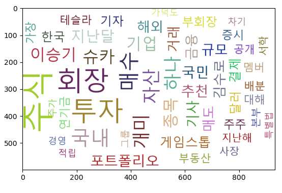
클라우드 차트
* nlp5.py
# 검색 결과를 형태소 분석하여 단어 빈도수를 구하고 이를 기초로 워드 클라우드 차트 출력
from bs4 import BeautifulSoup
import urllib.request
from urllib.parse import quote
#keyboard = input("검색어")
keyboard = "주식"
#print(quote(keyboard)) # encoding
# 동아일보 검색 기능
target_url ="https://www.donga.com/news/search?query=" + quote(keyboard)
print(target_url)
source_code = urllib.request.urlopen(target_url)
soup = BeautifulSoup(source_code, 'lxml', from_encoding='utf-8')
msg = ""
for title in soup.find_all("p", "tit"):
title_link = title.select("a")
#print(title_link)
article_url = title_link[0]['href'] # [<a href="https://www.donga.com/news/Issue/031407" target="_blank">독감<span cl ...
#print(article_url) # https://bizn.donga.com/3/all/20210226/105634947/2 ..
source_article = urllib.request.urlopen(article_url) # 실제 기사
soup = BeautifulSoup(source_article, 'lxml', from_encoding='utf-8')
cotents = soup.select('div.article_txt')
#print(cotents)
for temp in cotents:
item = str(temp.find_all(text=True))
#print(item)
msg = msg + item
print(msg)
from urllib.parse import quote
quote(문자열) : encoding
from konlpy.tag import Okt
from collections import Counter
nlp = Okt()
nouns = nlp.nouns(msg)
result = []
for temp in nouns:
if len(temp) > 1:
result.append(temp)
print(result)
print(len(result))
count = Counter(result)
print(count)
tag = count.most_common(50) # 상위 50개만 작업에 참여
anaconda prompt 실행
pip install simplejson
pip install pytagcloud